GWAS Meta analysis Using GXwasR
Banabithi Bose
University of Colorado Anschutz Medical;Northwestern Universitybanabithi.bose@gmail.com
16 October 2025
Source:vignettes/meta_analysis.Rmd
meta_analysis.RmdMeta analysis using GXwasR
Here we will present a tutorial showing how to perform meta analysis utilizing the R package GXwasR.
The example data sets for performing the tutorial can be accessed from “data” folder of the package.
Example Datasets
Example datasets are provided with the package and can be accessed by
calling the data() function.
Load the example datasets to perform this tutorial.
## Load library
library(GXwasR)
#>
#> GXwasR: Genome-wide and x-chromosome wide association analyses applying
#> best practices of quality control over genetic data
#> Version 0.99.0 () installed
#> Author: c(
#>     person(given = "Banabithi",
#>            family = "Bose",
#>            role = c("cre", "aut"),
#>            email = "banabithi.bose@gmail.com",
#>            comment = c(ORCID = "0000-0003-0842-8768"))
#>            )
#> Maintainer: Banabithi Bose <banabithi.bose@gmail.com>
#> Tutorial: https://github.com
#> Use citation("GXwasR") to know how to cite this work.- Two sets of summary GWAS summary statistics in .Rda files will be required to perform this tutorial.
- Summary_Stat_Ex1.Rda
- Summary_Stat_Ex2.Rda
Check one of the summary statistics data
data(Summary_Stat_Ex1)
## Visualize three rows and all the columns
Summary_Stat_Ex1[1:3, ]
#>   CHR         SNP     BP A1 TEST NMISS    BETA     SE     L95   U95    STAT
#> 1   1 rs143773730  73841  T  ADD   125 -0.0789 0.2643 -0.5968 0.439 -0.2986
#> 4   1 rs147281566 775125  T  ADD   125 -0.3959 1.2380 -2.8230 2.031 -0.3197
#> 6   1  rs35854196 863863  A  ADD   125  1.0500 0.8858 -0.6864 2.786  1.1850
#>        P
#> 1 0.7653
#> 4 0.7492
#> 6 0.2360
Among these 12 columns, some columns are mandatory for this tutorial, such as: ‘SNP’ (i.e., SNP identifier), ‘BETA’ (i.e., effect-size or logarithm of odds ratio), ‘SE’ (i.e., standard error of BETA), ‘P’ (i.e., p-values) and ‘NMISS’ (i.e., effective sample size). The other columns are, ‘CHR’ (i.e., chromosome code), ‘BP’ (i.e., base pair position), A1 (i.e., disease allele), TEST (i.e., association test type), L95 (i.e., lower limit of 95 percentile confidence interval), U95 (i.e., upper limit of 95 percentile confidence interval) and STAT (i.e., test statistic).
UniqueLoci.Rda: .Rda file with a single column containing SNP names. These could be LD clumped SNPs or any other list of chosen SNPs for Meta analysis.
SNPsPlot.Rda: .Rda file with a single column containing SNP names for the forest plots.
## Call some other libraries for this vignette
library(printr)
#> Registered S3 method overwritten by 'printr':
#>   method                from
#>   knit_print.data.frame rmarkdown
library(rmarkdown)
#>
#> Attaching package: 'rmarkdown'
#> The following objects are masked from 'package:BiocStyle':
#>
#>     html_document, md_document, pdf_document
The function for meta analysis:
MetaGWAS()
help(MetaGWAS, package = GXwasR)| MetaGWAS | R Documentation |
MetaGWAS: Combining summary-level results from two or more GWA studies into a single estimate.
Description
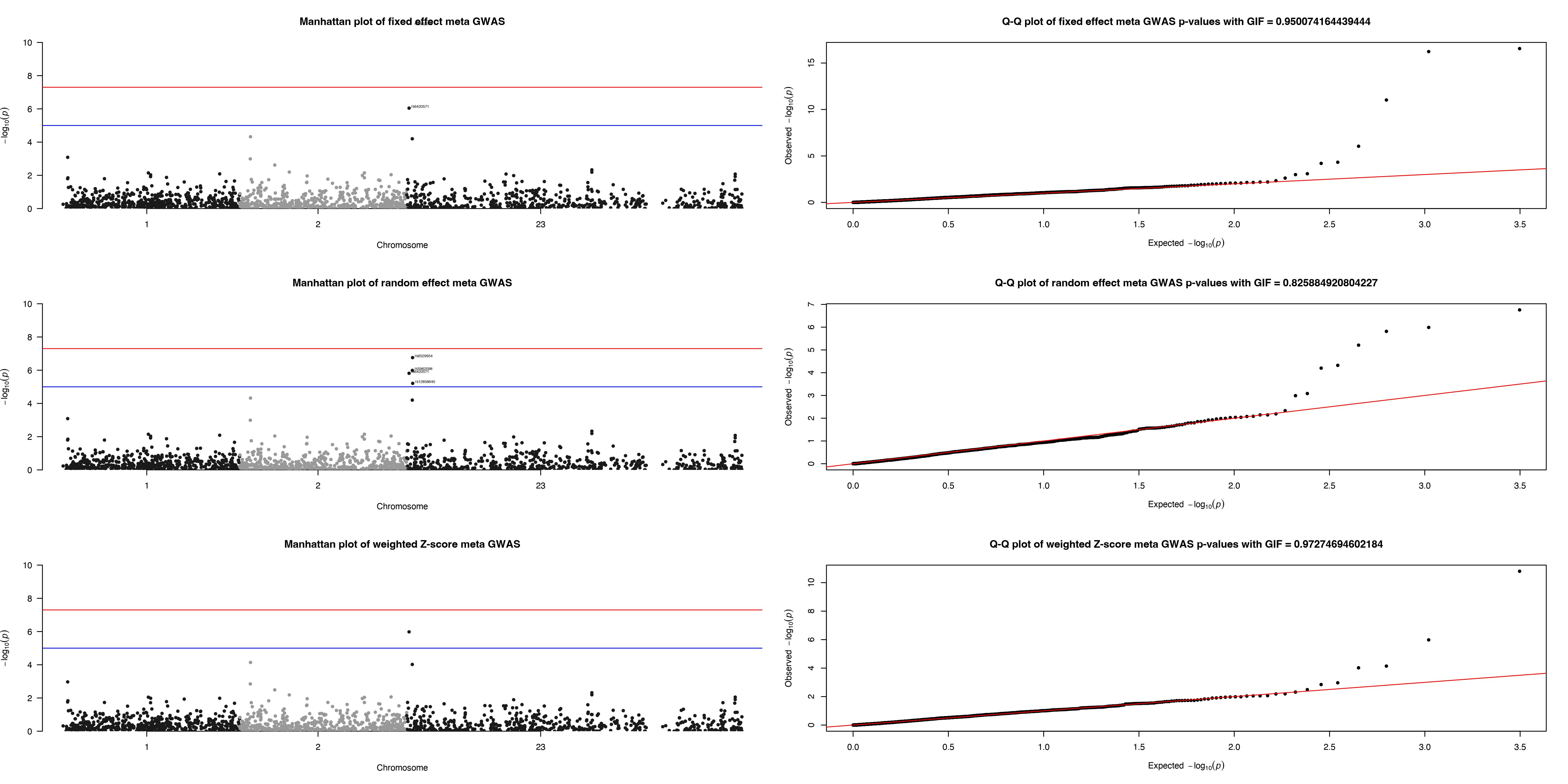
This function combine K sets of GWAS association statistics on same (or at least similar) phenotype. This function employs PLINK's (Purcell et al. 2007) inverse variance-based analysis to run a number of models, including a) Fixed-effect model and b) Random-effect model, assuming there may be variation between the genuine underlying effects, i.e., effect size beta. 'This function also calculates weighted Z-score-based p-values after METAL (Willer et al. 2010). For more information about the algorithms, please see the associated paper.
Usage
MetaGWAS(
  DataDir,
  SummData = c(""),
  ResultDir = tempdir(),
  SNPfile = NULL,
  useSNPposition = TRUE,
  UseA1 = FALSE,
  GCse = TRUE,
  plotname = "Meta_Analysis.plot",
  pval_filter = "R",
  top_snp_pval = 1e-08,
  max_top_snps = 6,
  chosen_snps_file = NULL,
  byCHR = FALSE,
  pval_threshold_manplot = 1e-05
)
Arguments
DataDir |
A character string for the file path of the input files needed for |
SummData |
Vector value containing the name(s) of the .Rda file(s) with GWAS summary statistics, with ‘SNP’
(i.e., SNP identifier), ‘BETA’ (i.e., effect-size or logarithm of odds ratio), ‘SE’ (i.e., standard error of BETA),
‘P’ (i.e., p-values), 'NMISS' (i.e., effective sample size), 'L95' (i.e., lower limit of 95% confidence interval) and
'U95' (i.e., upper limit of 95% confidence interval) are in mandatory column headers. These files needed to be in DataDir.
If the numbers of cases and controls are unequal, effective sample size should be |
ResultDir |
A character string for the file path where all output files will be stored. The default is |
SNPfile |
Character string specifying the name of the plain-text file with a column of SNP names. These could be LD clumped SNPs or
any other list of chosen SNPs for Meta analysis. This file needs to be in |
useSNPposition |
Boolean value, |
UseA1 |
Boolean value, |
GCse |
Boolean value, |
plotname |
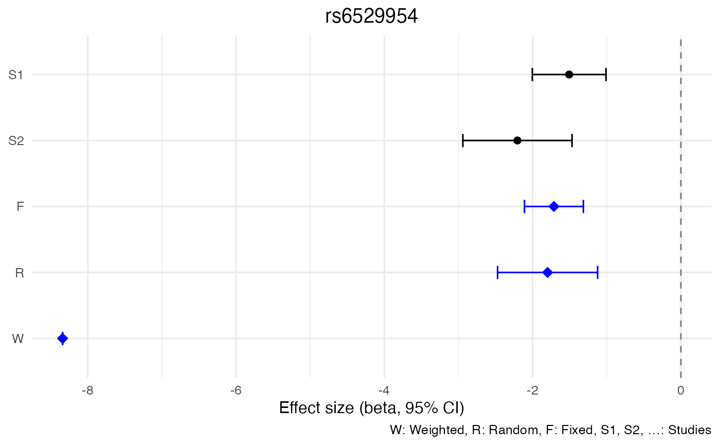
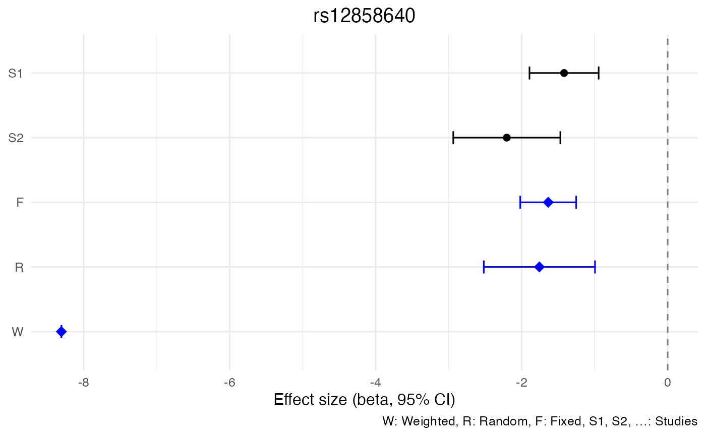
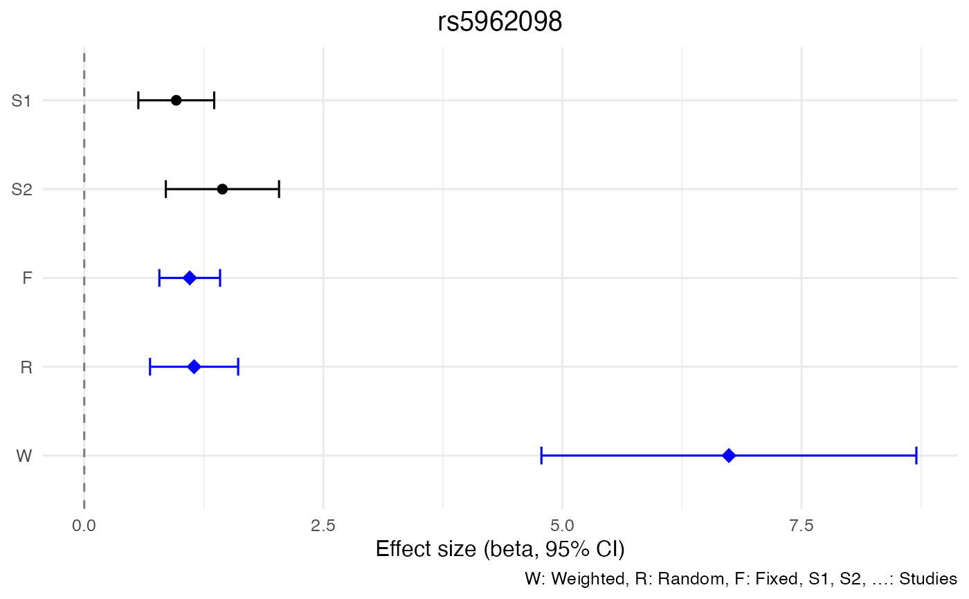
Character string, specifying the plot name of the file containing forest plots for the SNPs. The default is “Meta_Analysis.plot”. |
pval_filter |
Character value as "R","F" or "W", specifying whether p-value threshold should be chosen based on “Random”, “Fixed” or “Weighted” effect model for the SNPs to be included in the forest plots. |
top_snp_pval |
Numeric value, specifying the threshold to be used to filter the SNPs for the forest plots. The default is 1e-08. |
max_top_snps |
Integer value, specifying the maximum number of top SNPs (SNPs with the lowest p-values) to be ploted in the forest plot file. The default is 6. |
chosen_snps_file |
Character string specifying the name of the plain-text file with a column of SNP names for the forest plots. The default is NULL. |
byCHR |
Boolean value, |
pval_threshold_manplot |
Numeric value, specifying the p-value threshold for plotting Manhattan plots. |
Value
A list object containing five dataframes and a list of forest plots. The first three dataframes, such as Mfixed, Mrandom and Mweighted contain results for fixed effect, random effect and weighted model. Each of these dataframes can have maximum 12 columns, such as:
-
CHR(Chromosome code) -
BP(Basepair position) -
SNP(SNP identifier) -
A1(First allele code) -
A2(Second allele code) -
Q(p-value for Cochrane's Q statistic) -
I(I^2 heterogeneity index (0-100)) -
P(P-value from mata analysis) -
ES(Effect-size estimate from mata analysis) -
SE(Standard Error from mata analysis) -
CI_L(Lower limit of confidence interval) -
CI_U(Uper limit of confidence interval)
The fourth dataframe contains the same columns CHR, BP, SNP, A1, A2, Q, I", with column N' ( Number of
valid studies for this SNP), P (Fixed-effects meta-analysis p-value), and other columns as Fx... (Study x (0-based input file
indices) effect estimate, Examples: F0, F1 etc.).
The fifth dataframe, ProblemSNP has three columns, such as
-
File(file name of input data), -
SNP(Problematic SNPs that are thrown) -
Problem(Problem code)
Problem codes are:
-
BAD_CHR (Invalid chromosome code)
-
BAD_BP (Invalid base-position code), BAD_ES (Invalid effect-size)
-
BAD_SE (Invalid standard error), MISSING_A1 (Missing allele 1 label)
-
MISSING_A2 (Missing allele 2 label)
-
ALLELE_MISMATCH (Mismatching allele codes across files)
A .pdf file comprising the forest plots of the SNPs is produced in the ResultDir with Plotname as prefix.
If useSNPposition is set TRUE, a .jpeg file with Manhattan Plot and Q-Q plot will be in the ResultDir with Plotname
as prefix.
References
Purcell S, Neale B, Todd-Brown K, Thomas L, Ferreira MAR, Bender D, Maller J, Sklar P, de Bakker PIW, Daly MJ, others (2007).
“PLINK: A Tool Set for Whole-Genome Association and Population-Based Linkage Analyses.”
The American Journal of Human Genetics, 81(3), 559–575.
doi:10.1086/519795.
Willer CJ, Li Y, Abecasis GR (2010).
“METAL: fast and efficient meta-analysis of genomewide association scans.”
Bioinformatics, 26(17), 2190–2191.
doi:10.1093/bioinformatics/btq340, http://www.ncbi.nlm.nih.gov/pubmed/20616382.
Examples
data("Summary_Stat_Ex1", package = "GXwasR")
data("Summary_Stat_Ex2", package = "GXwasR")
DataDir <- GXwasR:::GXwasR_data()
ResultDir <- tempdir()
SummData <- list(Summary_Stat_Ex1, Summary_Stat_Ex2)
SNPfile <- "UniqueLoci"
useSNPposition <- FALSE
UseA1 <- TRUE
GCse <- TRUE
byCHR <- FALSE
pval_filter <- "R"
top_snp_pval <- 1e-08
max_top_snps <- 10
chosen_snps_file <- NULL
pval_threshold_manplot <- 1e-05
plotname <- "Meta_Analysis.plot"
x <- MetaGWAS(
    DataDir = DataDir, SummData = SummData, ResultDir = ResultDir,
    SNPfile = NULL, useSNPposition = TRUE, UseA1 = UseA1, GCse = GCse,
    plotname = "Meta_Analysis.plot", pval_filter, top_snp_pval, max_top_snps,
    chosen_snps_file = NULL, byCHR, pval_threshold_manplot
)
Running MetaGWAS
data(Summary_Stat_Ex1)
data(Summary_Stat_Ex2)
DataDir <- GXwasR:::GXwasR_data()
ResultDir <- tempdir()
SummData <- list(Summary_Stat_Ex1, Summary_Stat_Ex2)
SNPfile <- "UniqueLoci"
useSNPposition <- FALSE
UseA1 <- TRUE
GCse <- TRUE
byCHR <- FALSE
pval_filter <- "R"
top_snp_pval <- 1e-08
max_top_snps <- 10
chosen_snps_file <- NULL
pval_threshold_manplot <- 1e-05
plotname <- "Meta_Analysis.plot"

x <- MetaGWAS(DataDir = DataDir, SummData = SummData, ResultDir = ResultDir, SNPfile = NULL, useSNPposition = TRUE, UseA1 = UseA1, GCse = GCse, plotname = "Meta_Analysis.plot", pval_filter, top_snp_pval, max_top_snps, chosen_snps_file = NULL, byCHR, pval_threshold_manplot)
#> ℹ Processing file number 1
#> ℹ Processing file number 2
#> ℹ Applying study-specific genomic control.
#> ℹ Applying study-specific genomic control.
#> Processing chromosome
#> Using PLINK v1.9.0-b.7.7 64-bit (22 Oct 2024)
#> ✔ Forest plots for SNPS have compiled and saved as Meta_Analysis.plot.pdf
#> ℹ You can find them in the directory: /var/folders/d6/gtwl3_017sj4pp14fbfcbqjh0000gp/T//Rtmpqa0Y9k
#> ✔ Manhattan and QQ plots for SNPS have been compiled and saved as Meta_Analysis.plot.jpeg
#> ℹ You can find them in the directory: /var/folders/d6/gtwl3_017sj4pp14fbfcbqjh0000gp/T//Rtmpqa0Y9k
Random effect result
# Dataframe with the fixed effect result
x1 <- x$Resultrandom
x2 <- x1[order(x1$P), ]
knitr::kable(x2[1:10, ], caption = "Top ten associations from random effect model.")| CHR | BP | SNP | A1 | A2 | Q | I | P | ES | SE | CI_L | CI_U | |
|---|---|---|---|---|---|---|---|---|---|---|---|---|
| 1054 | 23 | 4184349 | rs6529954 | A | ? | 0.1162 | 59.48 | 0.0000002 | -1.7980 | 0.3441459 | -2.4725260 | -1.1234740 |
| 1053 | 23 | 4137114 | rs5962098 | A | ? | 0.1753 | 45.56 | 0.0000010 | 1.1488 | 0.2351018 | 0.6880004 | 1.6095996 |
| 1043 | 23 | 3376304 | rs6420571 | A | ? | 0.3068 | 4.26 | 0.0000015 | -1.1667 | 0.2426946 | -1.6423814 | -0.6910186 |
| 1055 | 23 | 4214861 | rs12858640 | C | ? | 0.0725 | 69.00 | 0.0000062 | -1.7572 | 0.3887229 | -2.5190968 | -0.9953032 |
| 559 | 2 | 2579014 | rs10186455 | G | ? | 0.4490 | 0.00 | 0.0000476 | 1.2694 | 0.3121061 | 0.6576721 | 1.8811279 |
| 1052 | 23 | 4119808 | rs10521557 | A | ? | 0.8021 | 0.00 | 0.0000631 | 1.4884 | 0.3720121 | 0.7592563 | 2.2175437 |
| 6 | 1 | 1127860 | rs148527527 | G | ? | 0.5778 | 0.00 | 0.0008237 | 1.3978 | 0.4179142 | 0.5786881 | 2.2169119 |
| 558 | 2 | 2535670 | rs13430614 | C | ? | 0.6681 | 0.00 | 0.0010230 | 0.6358 | 0.1935981 | 0.2563478 | 1.0152522 |
| 1382 | 23 | 45563626 | rs1207312 | T | ? | 0.5388 | 0.00 | 0.0046670 | 0.6138 | 0.2169547 | 0.1885689 | 1.0390311 |
| 1383 | 23 | 45565805 | rs1780835 | A | ? | 0.5206 | 0.00 | 0.0064620 | 0.5404 | 0.1984308 | 0.1514757 | 0.9293243 |
Fixed effect result
# Dataframe with the fixed effect result
x1 <- x$Resultfixed
x2 <- x1[order(x1$P), ]
knitr::kable(x2[1:10, ], caption = "Top ten associations from fixed effect model.")| CHR | BP | SNP | A1 | A2 | Q | I | P | ES | SE | CI_L | CI_U | |
|---|---|---|---|---|---|---|---|---|---|---|---|---|
| 1054 | 23 | 4184349 | rs6529954 | A | ? | 0.1162 | 59.48 | 0.0000000 | -1.7127 | 0.2025697 | -2.1097365 | -1.3156635 |
| 1055 | 23 | 4214861 | rs12858640 | C | ? | 0.0725 | 69.00 | 0.0000000 | -1.6364 | 0.1955735 | -2.0197240 | -1.2530760 |
| 1053 | 23 | 4137114 | rs5962098 | A | ? | 0.1753 | 45.56 | 0.0000000 | 1.1030 | 0.1618941 | 0.7856876 | 1.4203124 |
| 1043 | 23 | 3376304 | rs6420571 | A | ? | 0.3068 | 4.26 | 0.0000009 | -1.1647 | 0.2371161 | -1.6294476 | -0.6999524 |
| 559 | 2 | 2579014 | rs10186455 | G | ? | 0.4490 | 0.00 | 0.0000476 | 1.2694 | 0.3121061 | 0.6576721 | 1.8811279 |
| 1052 | 23 | 4119808 | rs10521557 | A | ? | 0.8021 | 0.00 | 0.0000631 | 1.4884 | 0.3720121 | 0.7592563 | 2.2175437 |
| 6 | 1 | 1127860 | rs148527527 | G | ? | 0.5778 | 0.00 | 0.0008237 | 1.3978 | 0.4179142 | 0.5786881 | 2.2169119 |
| 558 | 2 | 2535670 | rs13430614 | C | ? | 0.6681 | 0.00 | 0.0010230 | 0.6358 | 0.1935981 | 0.2563478 | 1.0152522 |
| 638 | 2 | 8181194 | rs7370955 | A | ? | 0.2403 | 27.48 | 0.0024130 | 0.7752 | 0.2555007 | 0.2744187 | 1.2759813 |
| 1382 | 23 | 45563626 | rs1207312 | T | ? | 0.5388 | 0.00 | 0.0046670 | 0.6138 | 0.2169547 | 0.1885689 | 1.0390311 |
Weighted effect result
# Dataframe with the fixed effect result
x1 <- x$Resultweighted
x2 <- x1[order(x1$P), ]
knitr::kable(x2[1:10, ], caption = "Top ten associations from weighted effect model.")| CHR | BP | SNP | A1 | A2 | Q | I | P | ES | SE | CI_L | CI_U | |
|---|---|---|---|---|---|---|---|---|---|---|---|---|
| 1054 | 23 | 4184349 | rs6529954 | A | ? | 0.1162 | 59.48 | 0.0000000 | -8.340 | 0.0000000 | -8.3400000 | -8.340000 |
| 1055 | 23 | 4214861 | rs12858640 | C | ? | 0.0725 | 69.00 | 0.0000000 | -8.306 | 0.0000000 | -8.3060000 | -8.306000 |
| 1053 | 23 | 4137114 | rs5962098 | A | ? | 0.1753 | 45.56 | 0.0000000 | 6.741 | 1.0000820 | 4.7808392 | 8.701161 |
| 1043 | 23 | 3376304 | rs6420571 | A | ? | 0.3068 | 4.26 | 0.0000010 | -4.883 | 1.0000062 | -6.8430122 | -2.922988 |
| 559 | 2 | 2579014 | rs10186455 | G | ? | 0.4490 | 0.00 | 0.0000723 | 3.969 | 1.0000874 | 2.0088287 | 5.929171 |
| 1052 | 23 | 4119808 | rs10521557 | A | ? | 0.8021 | 0.00 | 0.0000955 | 3.902 | 1.0000837 | 1.9418359 | 5.862164 |
| 6 | 1 | 1127860 | rs148527527 | G | ? | 0.5778 | 0.00 | 0.0010750 | 3.270 | 0.9999618 | 1.3100749 | 5.229925 |
| 558 | 2 | 2535670 | rs13430614 | C | ? | 0.6681 | 0.00 | 0.0014260 | 3.189 | 0.9998946 | 1.2292065 | 5.148794 |
| 638 | 2 | 8181194 | rs7370955 | A | ? | 0.2403 | 27.48 | 0.0032420 | 2.944 | 1.0000649 | 0.9838728 | 4.904127 |
| 1382 | 23 | 45563626 | rs1207312 | T | ? | 0.5388 | 0.00 | 0.0048350 | 2.818 | 1.0000617 | 0.8578790 | 4.778121 |
Metadata of the meta analysis
# Dataframe with the metadata
x1 <- x$Metadata
x2 <- x1[order(x1$Q), ]
knitr::kable(x2[1:10, ], caption = "Metadata of the top ten associations based on Cochrane’s Q statistics.")| CHR | BP | SNP | A1 | A2 | N | Q | I | F0 | F1 | |
|---|---|---|---|---|---|---|---|---|---|---|
| 812 | 2 | 21385538 | rs575905 | T | ? | 2 | 0.0010 | 90.73 | -0.5218 | 0.6472 |
| 1110 | 23 | 9277424 | rs2214279 | G | ? | 2 | 0.0015 | 90.09 | 0.5001 | -0.5365 |
| 655 | 2 | 9913645 | rs1106144 | A | ? | 2 | 0.0020 | 89.48 | 0.5909 | -0.8972 |
| 663 | 2 | 10210922 | rs11678624 | T | ? | 2 | 0.0021 | 89.45 | -0.3659 | 0.7374 |
| 1207 | 23 | 23909933 | rs2428144 | A | ? | 2 | 0.0031 | 88.55 | 0.5344 | -0.4081 |
| 1253 | 23 | 29189630 | rs225456 | C | ? | 2 | 0.0031 | 88.56 | 0.3208 | -1.1170 |
| 1248 | 23 | 28763567 | rs12008039 | G | ? | 2 | 0.0032 | 88.48 | -0.3187 | 0.5565 |
| 810 | 2 | 21275825 | rs12468735 | A | ? | 2 | 0.0036 | 88.19 | -0.5095 | 0.5175 |
| 664 | 2 | 10343419 | rs759347 | C | ? | 2 | 0.0041 | 87.88 | 0.9790 | -0.3894 |
| 1251 | 23 | 29104124 | rs16988439 | C | ? | 2 | 0.0042 | 87.81 | 0.3208 | -1.0730 |
Problematic SNPs
# Dataframe with the problematic SNPs
x1 <- x$ProblemSNP
knitr::kable(x1[1:10, ], caption = "Top ten problematic SNPs.")| File | SNP | Problem |
|---|---|---|
| /private/var/folders/d6/gtwl3_017sj4pp14fbfcbqjh0000gp/T/Rtmpqa0Y9k/SNPdata_2 | rs2803333 | ALLELE_MISMATCH |
| /private/var/folders/d6/gtwl3_017sj4pp14fbfcbqjh0000gp/T/Rtmpqa0Y9k/SNPdata_2 | rs672606 | ALLELE_MISMATCH |
| /private/var/folders/d6/gtwl3_017sj4pp14fbfcbqjh0000gp/T/Rtmpqa0Y9k/SNPdata_2 | rs7519955 | ALLELE_MISMATCH |
| /private/var/folders/d6/gtwl3_017sj4pp14fbfcbqjh0000gp/T/Rtmpqa0Y9k/SNPdata_2 | rs1538466 | ALLELE_MISMATCH |
| /private/var/folders/d6/gtwl3_017sj4pp14fbfcbqjh0000gp/T/Rtmpqa0Y9k/SNPdata_2 | rs61777960 | ALLELE_MISMATCH |
| /private/var/folders/d6/gtwl3_017sj4pp14fbfcbqjh0000gp/T/Rtmpqa0Y9k/SNPdata_2 | rs2865211 | ALLELE_MISMATCH |
| /private/var/folders/d6/gtwl3_017sj4pp14fbfcbqjh0000gp/T/Rtmpqa0Y9k/SNPdata_2 | rs10917217 | ALLELE_MISMATCH |
| /private/var/folders/d6/gtwl3_017sj4pp14fbfcbqjh0000gp/T/Rtmpqa0Y9k/SNPdata_2 | rs196402 | ALLELE_MISMATCH |
| /private/var/folders/d6/gtwl3_017sj4pp14fbfcbqjh0000gp/T/Rtmpqa0Y9k/SNPdata_2 | rs6662038 | ALLELE_MISMATCH |
| /private/var/folders/d6/gtwl3_017sj4pp14fbfcbqjh0000gp/T/Rtmpqa0Y9k/SNPdata_2 | rs3845484 | ALLELE_MISMATCH |
Reproducibility
The GXwasR package (Bose, Blostein, Kim, Winters, Actkins, Mayer, Congivaram, Niarchou, Edwards, Davis, and Stranger, 2025) was made possible thanks to:
- R (R Core Team, 2025)
- BiocStyle (Oleś, 2025)
- knitr (Xie, 2025)
- RefManageR (McLean, 2017)
- rmarkdown (Allaire, Xie, Dervieux, McPherson, Luraschi, Ushey, Atkins, Wickham, Cheng, Chang, and Iannone, 2025)
- sessioninfo (Wickham, Chang, Flight, Müller, and Hester, 2025)
- testthat (Wickham, 2011)
This package was developed using biocthis.
R session information.
#> ─ Session info ───────────────────────────────────────────────────────────────────────────────────────────────────────
#>  setting  value
#>  version  R version 4.5.1 (2025-06-13)
#>  os       macOS Sequoia 15.7.1
#>  system   aarch64, darwin24.4.0
#>  ui       unknown
#>  language en-US
#>  collate  en_US.UTF-8
#>  ctype    en_US.UTF-8
#>  tz       America/New_York
#>  date     2025-10-16
#>  pandoc   3.6.3 @ /Applications/Positron.app/Contents/Resources/app/quarto/bin/tools/aarch64/ (via rmarkdown)
#>  quarto   1.8.25 @ /usr/local/bin/quarto
#>
#> ─ Packages ───────────────────────────────────────────────────────────────────────────────────────────────────────────
#>  package              * version   date (UTC) lib source
#>  abind                  1.4-8     2024-09-12 [1] CRAN (R 4.5.0)
#>  backports              1.5.0     2024-05-23 [1] CRAN (R 4.5.1)
#>  bibtex                 0.5.1     2023-01-26 [1] CRAN (R 4.5.0)
#>  bigassertr             0.1.7     2025-06-27 [1] CRAN (R 4.5.1)
#>  bigparallelr           0.3.2     2021-10-02 [1] CRAN (R 4.5.0)
#>  bigsnpr                1.12.21   2025-08-21 [1] CRAN (R 4.5.1)
#>  bigsparser             0.7.3     2024-09-06 [1] CRAN (R 4.5.1)
#>  bigstatsr              1.6.2     2025-07-29 [1] CRAN (R 4.5.1)
#>  Biobase                2.68.0    2025-04-15 [1] Bioconduc~
#>  BiocGenerics           0.54.0    2025-04-15 [1] Bioconduc~
#>  BiocIO                 1.18.0    2025-04-15 [1] Bioconduc~
#>  BiocManager            1.30.26   2025-06-05 [1] CRAN (R 4.5.0)
#>  BiocParallel           1.42.2    2025-09-14 [1] Bioconductor 3.21 (R 4.5.1)
#>  BiocStyle            * 2.36.0    2025-04-15 [1] Bioconduc~
#>  Biostrings             2.76.0    2025-04-15 [1] Bioconduc~
#>  bit                    4.6.0     2025-03-06 [1] CRAN (R 4.5.1)
#>  bit64                  4.6.0-1   2025-01-16 [1] CRAN (R 4.5.1)
#>  bitops                 1.0-9     2024-10-03 [1] CRAN (R 4.5.0)
#>  bookdown               0.45      2025-10-03 [1] CRAN (R 4.5.1)
#>  broom                  1.0.10    2025-09-13 [1] CRAN (R 4.5.1)
#>  BSgenome               1.76.0    2025-04-15 [1] Bioconduc~
#>  bslib                  0.9.0     2025-01-30 [1] CRAN (R 4.5.0)
#>  cachem                 1.1.0     2024-05-16 [1] CRAN (R 4.5.0)
#>  calibrate              1.7.7     2020-06-19 [1] CRAN (R 4.5.0)
#>  car                    3.1-3     2024-09-27 [1] CRAN (R 4.5.0)
#>  carData                3.0-5     2022-01-06 [1] CRAN (R 4.5.0)
#>  cli                    3.6.5     2025-04-23 [1] CRAN (R 4.5.0)
#>  codetools              0.2-20    2024-03-31 [3] CRAN (R 4.5.1)
#>  cowplot                1.2.0     2025-07-07 [1] CRAN (R 4.5.1)
#>  crayon                 1.5.3     2024-06-20 [1] CRAN (R 4.5.0)
#>  curl                   7.0.0     2025-08-19 [1] CRAN (R 4.5.1)
#>  data.table             1.17.8    2025-07-10 [1] CRAN (R 4.5.1)
#>  DelayedArray           0.34.1    2025-04-17 [1] Bioconduc~
#>  desc                   1.4.3     2023-12-10 [1] CRAN (R 4.5.0)
#>  digest                 0.6.37    2024-08-19 [1] CRAN (R 4.5.0)
#>  doParallel             1.0.17    2022-02-07 [1] CRAN (R 4.5.0)
#>  doRNG                  1.8.6.2   2025-04-02 [1] CRAN (R 4.5.0)
#>  dplyr                  1.1.4     2023-11-17 [1] CRAN (R 4.5.0)
#>  evaluate               1.0.5     2025-08-27 [1] CRAN (R 4.5.1)
#>  farver                 2.1.2     2024-05-13 [1] CRAN (R 4.5.0)
#>  fastmap                1.2.0     2024-05-15 [1] CRAN (R 4.5.0)
#>  flock                  0.7       2016-11-12 [1] CRAN (R 4.5.1)
#>  foreach                1.5.2     2022-02-02 [1] CRAN (R 4.5.0)
#>  Formula                1.2-5     2023-02-24 [1] CRAN (R 4.5.0)
#>  fs                     1.6.6     2025-04-12 [1] CRAN (R 4.5.0)
#>  gdsfmt                 1.44.1    2025-07-09 [1] Bioconduc~
#>  generics               0.1.4     2025-05-09 [1] CRAN (R 4.5.0)
#>  GenomeInfoDb           1.44.3    2025-09-21 [1] Bioconductor 3.21 (R 4.5.1)
#>  GenomeInfoDbData       1.2.14    2025-04-21 [1] Bioconductor
#>  GenomicAlignments      1.44.0    2025-04-15 [1] Bioconduc~
#>  GenomicRanges          1.60.0    2025-04-15 [1] Bioconduc~
#>  ggplot2                4.0.0     2025-09-11 [1] CRAN (R 4.5.1)
#>  ggpubr                 0.6.1     2025-06-27 [1] CRAN (R 4.5.1)
#>  ggrepel                0.9.6     2024-09-07 [1] CRAN (R 4.5.1)
#>  ggsignif               0.6.4     2022-10-13 [1] CRAN (R 4.5.0)
#>  glue                   1.8.0     2024-09-30 [1] CRAN (R 4.5.0)
#>  gridExtra              2.3       2017-09-09 [1] CRAN (R 4.5.0)
#>  gtable                 0.3.6     2024-10-25 [1] CRAN (R 4.5.0)
#>  GXwasR               * 0.99.0    2025-10-02 [1] Bioconductor
#>  hms                    1.1.3     2023-03-21 [1] CRAN (R 4.5.0)
#>  htmltools              0.5.8.1   2024-04-04 [1] CRAN (R 4.5.0)
#>  htmlwidgets            1.6.4     2023-12-06 [1] CRAN (R 4.5.0)
#>  httr                   1.4.7     2023-08-15 [1] CRAN (R 4.5.0)
#>  IRanges                2.42.0    2025-04-15 [1] Bioconduc~
#>  iterators              1.0.14    2022-02-05 [1] CRAN (R 4.5.0)
#>  jpeg                   0.1-11    2025-03-21 [1] CRAN (R 4.5.0)
#>  jquerylib              0.1.4     2021-04-26 [1] CRAN (R 4.5.0)
#>  jsonlite               2.0.0     2025-03-27 [1] CRAN (R 4.5.0)
#>  knitr                  1.50      2025-03-16 [1] CRAN (R 4.5.0)
#>  labeling               0.4.3     2023-08-29 [1] CRAN (R 4.5.0)
#>  lattice                0.22-7    2025-04-02 [3] CRAN (R 4.5.1)
#>  lifecycle              1.0.4     2023-11-07 [1] CRAN (R 4.5.0)
#>  lubridate              1.9.4     2024-12-08 [1] CRAN (R 4.5.1)
#>  magrittr               2.0.4     2025-09-12 [1] CRAN (R 4.5.1)
#>  MASS                   7.3-65    2025-02-28 [3] CRAN (R 4.5.1)
#>  mathjaxr               1.8-0     2025-04-30 [1] CRAN (R 4.5.1)
#>  Matrix                 1.7-4     2025-08-28 [3] CRAN (R 4.5.1)
#>  MatrixGenerics         1.20.0    2025-04-15 [1] Bioconduc~
#>  matrixStats            1.5.0     2025-01-07 [1] CRAN (R 4.5.0)
#>  memoise                2.0.1     2021-11-26 [1] CRAN (R 4.5.0)
#>  pillar                 1.11.1    2025-09-17 [1] CRAN (R 4.5.1)
#>  pkgconfig              2.0.3     2019-09-22 [1] CRAN (R 4.5.0)
#>  pkgdown                2.1.3     2025-05-25 [2] CRAN (R 4.5.0)
#>  plyr                   1.8.9     2023-10-02 [1] CRAN (R 4.5.1)
#>  plyranges              1.28.0    2025-04-15 [1] Bioconduc~
#>  poolr                  1.2-0     2025-05-07 [1] CRAN (R 4.5.0)
#>  prettyunits            1.2.0     2023-09-24 [1] CRAN (R 4.5.0)
#>  printr               * 0.3       2023-03-08 [1] CRAN (R 4.5.0)
#>  progress               1.2.3     2023-12-06 [1] CRAN (R 4.5.0)
#>  purrr                  1.1.0     2025-07-10 [1] CRAN (R 4.5.1)
#>  qqman                  0.1.9     2023-08-23 [1] CRAN (R 4.5.0)
#>  R.methodsS3            1.8.2     2022-06-13 [1] CRAN (R 4.5.0)
#>  R.oo                   1.27.1    2025-05-02 [1] CRAN (R 4.5.0)
#>  R.utils                2.13.0    2025-02-24 [1] CRAN (R 4.5.0)
#>  R6                     2.6.1     2025-02-15 [1] CRAN (R 4.5.0)
#>  ragg                   1.5.0     2025-09-02 [2] CRAN (R 4.5.1)
#>  rbibutils              2.3       2024-10-04 [1] CRAN (R 4.5.1)
#>  RColorBrewer           1.1-3     2022-04-03 [1] CRAN (R 4.5.0)
#>  Rcpp                   1.1.0     2025-07-02 [1] CRAN (R 4.5.1)
#>  RCurl                  1.98-1.17 2025-03-22 [1] CRAN (R 4.5.0)
#>  Rdpack                 2.6.4     2025-04-09 [1] CRAN (R 4.5.0)
#>  RefManageR           * 1.4.0     2022-09-30 [1] CRAN (R 4.5.1)
#>  regioneR               1.40.1    2025-06-01 [1] Bioconductor 3.21 (R 4.5.0)
#>  restfulr               0.0.16    2025-06-27 [1] CRAN (R 4.5.1)
#>  rjson                  0.2.23    2024-09-16 [1] CRAN (R 4.5.0)
#>  rlang                  1.1.6     2025-04-11 [1] CRAN (R 4.5.0)
#>  rmarkdown            * 2.30      2025-09-28 [1] CRAN (R 4.5.1)
#>  rmio                   0.4.0     2022-02-17 [1] CRAN (R 4.5.0)
#>  rngtools               1.5.2     2021-09-20 [1] CRAN (R 4.5.0)
#>  Rsamtools              2.24.1    2025-09-07 [1] Bioconductor 3.21 (R 4.5.1)
#>  rstatix                0.7.2     2023-02-01 [1] CRAN (R 4.5.0)
#>  rtracklayer            1.68.0    2025-04-15 [1] Bioconduc~
#>  S4Arrays               1.8.1     2025-06-01 [1] Bioconductor 3.21 (R 4.5.0)
#>  S4Vectors              0.46.0    2025-04-15 [1] Bioconduc~
#>  S7                     0.2.0     2024-11-07 [1] CRAN (R 4.5.1)
#>  sass                   0.4.10    2025-04-11 [1] CRAN (R 4.5.0)
#>  scales                 1.4.0     2025-04-24 [1] CRAN (R 4.5.0)
#>  sessioninfo          * 1.2.3     2025-02-05 [1] CRAN (R 4.5.1)
#>  SNPRelate              1.42.0    2025-04-15 [1] Bioconduc~
#>  SparseArray            1.8.1     2025-07-23 [1] Bioconduc~
#>  stringi                1.8.7     2025-03-27 [1] CRAN (R 4.5.0)
#>  stringr                1.5.2     2025-09-08 [1] CRAN (R 4.5.1)
#>  sumFREGAT              1.2.5     2022-06-07 [1] CRAN (R 4.5.1)
#>  SummarizedExperiment   1.38.1    2025-04-30 [1] Bioconductor 3.21 (R 4.5.0)
#>  sys                    3.4.3     2024-10-04 [1] CRAN (R 4.5.0)
#>  systemfonts            1.3.1     2025-10-01 [1] CRAN (R 4.5.1)
#>  textshaping            1.0.3     2025-09-02 [1] CRAN (R 4.5.1)
#>  tibble                 3.3.0     2025-06-08 [1] CRAN (R 4.5.0)
#>  tidyr                  1.3.1     2024-01-24 [1] CRAN (R 4.5.1)
#>  tidyselect             1.2.1     2024-03-11 [1] CRAN (R 4.5.0)
#>  timechange             0.3.0     2024-01-18 [1] CRAN (R 4.5.1)
#>  tzdb                   0.5.0     2025-03-15 [1] CRAN (R 4.5.1)
#>  UCSC.utils             1.4.0     2025-04-15 [1] Bioconduc~
#>  vctrs                  0.6.5     2023-12-01 [1] CRAN (R 4.5.0)
#>  vroom                  1.6.6     2025-09-19 [1] CRAN (R 4.5.1)
#>  withr                  3.0.2     2024-10-28 [1] CRAN (R 4.5.0)
#>  xfun                   0.53      2025-08-19 [1] CRAN (R 4.5.1)
#>  XML                    3.99-0.19 2025-08-22 [1] CRAN (R 4.5.1)
#>  xml2                   1.4.0     2025-08-20 [1] CRAN (R 4.5.1)
#>  XVector                0.48.0    2025-04-15 [1] Bioconduc~
#>  yaml                   2.3.10    2024-07-26 [1] CRAN (R 4.5.0)
#>
#>  [1] /Users/mayerdav/Library/R/arm64/4.5/library
#>  [2] /opt/homebrew/lib/R/4.5/site-library
#>  [3] /opt/homebrew/Cellar/r/4.5.1/lib/R/library
#>  * ── Packages attached to the search path.
#>
#> ──────────────────────────────────────────────────────────────────────────────────────────────────────────────────────
Bibliography
This vignette was generated using BiocStyle (Oleś, 2025) with knitr (Xie, 2025) and rmarkdown (Allaire, Xie, Dervieux et al., 2025) running behind the scenes.
Citations made with RefManageR (McLean, 2017).
[1] J. Allaire, Y. Xie, C. Dervieux, et al. rmarkdown: Dynamic Documents for R. R package version 2.30. 2025. URL: https://github.com/rstudio/rmarkdown.
[2] B. Bose, F. Blostein, J. Kim, et al. “GXwasR: A Toolkit for Investigating Sex-Differentiated Genetic Effects on Complex Traits”. In: medRxiv 2025.06.10.25329327 (2025). DOI: 10.1101/2025.06.10.25329327.
[3] M. W. McLean. “RefManageR: Import and Manage BibTeX and BibLaTeX References in R”. In: The Journal of Open Source Software (2017). DOI: 10.21105/joss.00338.
[4] A. Oleś. BiocStyle: Standard styles for vignettes and other Bioconductor documents. R package version 2.36.0. 2025. DOI: 10.18129/B9.bioc.BiocStyle. URL: https://bioconductor.org/packages/BiocStyle.
[5] R Core Team. R: A Language and Environment for Statistical Computing. R Foundation for Statistical Computing. Vienna, Austria, 2025. URL: https://www.R-project.org/.
[6] H. Wickham. “testthat: Get Started with Testing”. In: The R Journal 3 (2011), pp. 5–10. URL: https://journal.r-project.org/archive/2011-1/RJournal_2011-1_Wickham.pdf.
[7] H. Wickham, W. Chang, R. Flight, et al. sessioninfo: R Session Information. R package version 1.2.3. 2025. DOI: 10.32614/CRAN.package.sessioninfo. URL: https://CRAN.R-project.org/package=sessioninfo.
[8] Y. Xie. knitr: A General-Purpose Package for Dynamic Report Generation in R. R package version 1.50. 2025. URL: https://yihui.org/knitr/.