Running GWAS, XWAS and Sex-differential tests Using GXwasR

Introduction

This document contains an example of running a GWAS with XWAS model and Sex-differential tests.

Users must perform pre-imputation and post-imputation quality control (QC) on genotype dataset and then proceed with this tutorial in actual scenario. Please follow the detailed QC-ed steps provided in: GXwasR_Preimputation and GXwasR_Postimputation.

Example Datasets

The PLINK bed, bim, and fam files are the three mandatory files representing a genotype dataset to run this tutorial. To know about these file extensions, please check https://www.cog-genomics.org/plink/1.9/formats.

GXwasR_example:

GXwasR_example.bed
GXwasR_example.bim
GXwasR_example.fam

These plink files contain genotypes for 276 individuals (males and females) simulated from 1000Genome from European decent with 26515 variants across twelve chromosomes (1-10,23,24). This dataset contains 125 males, 151 females, 108 cases and 168 controls. We will utilize this set of plink files as proxy of pre-imputated genotype data.

Loading the GXwasR library

## Call some libraries
library(GXwasR)
#> 
#> GXwasR: Genome-wide and x-chromosome wide association analyses applying
#> best practices of quality control over genetic data
#> Version 0.99.0 () installed
#> Author: c(
#>     person(given = "Banabithi",
#>            family = "Bose",
#>            role = c("cre", "aut"),
#>            email = "banabithi.bose@gmail.com",
#>            comment = c(ORCID = "0000-0003-0842-8768"))
#>            )
#> Maintainer: Banabithi Bose <banabithi.bose@gmail.com>
#> Tutorial: https://github.com
#> Use citation("GXwasR") to know how to cite this work.
library(printr)
#> Registered S3 method overwritten by 'printr':
#>   method                from     
#>   knit_print.data.frame rmarkdown
library(rmarkdown)
#> 
#> Attaching package: 'rmarkdown'
#> The following objects are masked from 'package:BiocStyle':
#> 
#>     html_document, md_document, pdf_document

Learn about all the GXwasR functions

browseVignettes("GXwasR")

Example Dataset Summary

Dataset: GXwasR_example

DataDir <- GXwasR:::GXwasR_data()
ResultDir <- tempdir()
finput <- "GXwasR_example"
x <- PlinkSummary(DataDir, ResultDir, finput)
#> ℹ Dataset: GXwasR_example
#> ℹ Number of missing phenotypes: 0
#> ℹ Number of males: 125
#> ℹ Number of females: 151
#> ℹ This is case-control data
#> ℹ Number of cases: 108
#> ℹ Number of controls: 168
#> ℹ Number of cases in males: 53
#> ℹ Number of controls in males: 72
#> ℹ Number of cases in females: 55
#> ℹ Number of controls in females: 96
#> ℹ Number of chromosomes: 12
#>   - Chr: 1
#>   - Chr: 2
#>   - Chr: 3
#>   - Chr: 4
#>   - Chr: 5
#>   - Chr: 6
#>   - Chr: 7
#>   - Chr: 8
#>   - Chr: 9
#>   - Chr: 10
#>   - Chr: 23
#>   - Chr: 24
#> ℹ Total number of SNPs: 26527
#> ℹ Total number of samples: 276

Sex-combined and sex-stratified GWAS with XWAS

Function: GXwas()

help(GXwas, package = GXwasR)

GXwas

R Documentation

GXwas: Running genome-wide association study (GWAS) and X-chromosome-wide association study (XWAS) models.

Description

This function runs GWAS models in autosomes with several alternative XWAS models. Models such as "FMcombx01","FMcombx02",and "FMstratified" can be applied to both binary and quantitative traits, while "GWAcxci" can only be applied to a binary trait.

For binary and quantitative features, this function uses logistic and linear regression, allowing for multiple covariates and the interactions with those covariates in a multiple-regression approach. These models are all run using the additive effects of SNPs, and each additional minor allele's influence is represented by the direction of the regression coefficient.

This function attempts to identify the multi-collinearity among predictors by displaying NA for the test statistic and a p-value for all terms in the model. The more terms you add, the more likely you are to run into issues.

For details about the different XWAS model, please follow the associated publication.

Usage

GXwas(
  DataDir,
  ResultDir,
  finput,
  trait = c("binary", "quantitative"),
  standard_beta = TRUE,
  xmodel = c("FMcombx01", "FMcombx02", "FMstratified", "GWAScxci"),
  sex = FALSE,
  xsex = FALSE,
  covarfile = NULL,
  interaction = FALSE,
  covartest = c("ALL"),
  Inphenocov = c("ALL"),
  combtest = c("fisher.method", "fisher.method.perm", "stouffer.method"),
  MF.zero.sub = 1e-05,
  B = 10000,
  MF.mc.cores = 1,
  MF.na.rm = FALSE,
  MF.p.corr = "none",
  plot.jpeg = FALSE,
  plotname = "GXwas.plot",
  snp_pval = 1e-08,
  annotateTopSnp = FALSE,
  suggestiveline = 5,
  genomewideline = 7.3,
  ncores = 0
)

Arguments

DataDir

Character string for the file path of the input PLINK binary files.

ResultDir

Character string for the folder path where the outputs will be saved.

finput

Character string, specifying the prefix of the input PLINK binary files with both male and female samples. This file needs to be in DataDir.

Note: Case/control phenotypes are expected to be encoded as 1=unaffected (control), 2=affected (case); 0 is accepted as an alternate missing value encoding. The missing case/control or quantitative phenotypes are expected to be encoded as 'NA'/'nan' (any capitalization) or -9.

trait

Boolean value, 'binary' or 'quantitative' for the phenotype i.e. the trait.

standard_beta

Boolean value, TRUE or FALSE in case of quantitative trait for standardizing the trait or phenotype values (mean 0, unit variance), so the resulting coefficients will be standardized. The default is TRUE.

xmodel

Models "FMcombx01","FMcombx02",and "FMstratified" can be chosen for both binary and quantitative traits while "GWAcxci" can only apply to the binary trait. These models take care of the X-chromosomal marker. Three female genotypes are coded by 0, 1, and 2 in FM01 and FM02. The two genotypes of males that follow the X-chromosome inactivation (XCI) pattern as random (XCI-R) in the FM01 model are coded by 0 and 1, while the two genotypes that follow the XCI is escaped (XCI-E) in the FM02 model are coded by 0 and 1. To reflect the dose compensation connection between the sexes, FM02 treats men as homozygous females.

In the "FMstratified" associations are tested separately for males and females, and then the combined p values are computed the Fisher's method, Fisher's method with permutation, or Stouffer's method(1,3-7]. An X-chromosome inactivation (XCI) pattern, or coding technique for X-chromosomal genotypes between sexes, is not required for the XCGA. By simultaneously accounting for four distinct XCI patterns, namely XCI-R, XCI-E, XCI-SN (XCI fully toward normal allele), and XCI-SR (XCI fully toward risk allele), this model may maintain a respectably high power (Su et al. 2022).

Note: sex shouldn't be provided as a covariate in the XCGA model.

sex

Boolean value, TRUE or FALSE for using sex as covariate in association test. It is applicable genome-wide.

The default is FALSE.

xsex

Boolean value, TRUE or FALSE for using sex as covariate in association test for X-chromosomal SNPs. The default is FALSE. This will overwrite 'sex' argument for X-chromosome.

covarfile

Character string for the full name of the covariate file in .txt format. This file should be placed in DataDir.

Note about the covariate file: The first column of this file should be FID, the second column should be IID and the other columns should be covariates. The primary header line should be there starting with “FID”, and “IID” followed by covariate names. If an individual is not present in the covariate file, or if the individual has a missing phenotype value (i.e. -9 by default) for the covariate, then that individual is set to missing (i.e. will be excluded from association analysis). It is important to note that for stratified GWAS model, if PCs are included as covar then it should be generated separately for each cohort and then included in the covarfile. Use the function DummyCovar to generate a new covariate file with categorical variables down-coded as binary dummy variables for the covariate file with categorical variables. For instance, if a variable has K categories, K-1 new dummy variables are constructed, and the original covariate is now estimated with a coefficient for each category.

interaction

Boolean value, TRUE or FALSE for including SNP x covariate interaction term/terms from the association analysis. The default is FALSE. If a permutation procedure is chosen then the interaction will be automatically FALSE. For the interaction with the two covariates COV1 and COV2, the model will look like: Y = b0 + b1.ADD + b2.COV1 + b3.COV2 + b4.ADD x COV1 + b5.ADD x COV2 + e. When interaction factors are incorporated into the model, the main effects' significance is not always determined simply; rather, it depends on the arbitrary coding of the variables. To put it another way, you should probably just interpret the p-value for the interaction. Also, The p-values for the covariates do not represent the test for the SNP-phenotype association after controlling for the covariate. That is the first row (ADD). Rather, the covariate term is the test associated with the covariate-phenotype association. These p-values might be extremely significant (e.g. if one covaries for smoking in an analysis of heart disease, etc) but this does not mean that the SNP has a highly significant effect necessarily. Note that, this feature is not valid for XCGA model for XWAS part.

covartest

Vector value with NULL,"ALL" or covariate name/names to be included in the test. The default is NULL. For instance, the user can choose “AGE” and “SEX” as covartest = c(“AGE”, “SEX”) or all the covariates as covartest = c(“ALL”).

Inphenocov

Vector of integer values starting from 1 to extract the terms which user wants from the above model: Y = b0 + b1.ADD + b2.COV1 + b3.COV2 + b4.ADDxCOV1 + b5.ADDxCOV2 + e. The terms will appear in order as (Purcell et al. 2007) for ADD, (Su et al. 2022) for COV1, (Rhodes 2002) for ADD x COV1, and (Moreau and others 2003) for ADD x COV2. If the user wants to extract the terms for COV1 and ADD x COV1, they need to specify it as c(2,4). The default is ⁠c(“ALL”)⁠.

Note: This feature is not valid for the XCGA model for the XWAS part.

combtest

Character vector specifying method for combining p-values after stratified GWAS/XWAS models. Choices are “stouffer.method”, "fisher.method" and "fisher.method.perm". For fisher.method the function for combining p-values uses a statistic, S = -2 ∑^k /log p, which follows a χ^2 distribution with 2k degrees of freedom (Fisher 1925).

For fisher.method.perm, using p-values from stratified tests, the summary statistic for combining p-values is S = -2 ∑ /log p. A p-value for this statistic can be derived by randomly generating summary statistics (Rhodes 2002). Therefore, a p-value is randomly sampled from each contributing study, and a random statistic is calculated. The fraction of random statistics greater or equal to S then gives the final p-value.

For stouffer.method ,the function applies Stouffer’s method (Stouffer et al. 1949) to the p-values assuming that the p-values to be combined are independent. Letting p1, p2, . . . , pk denote the individual (one- or two-sided) p-values of the k hypothesis tests to be combined, the test statistic is then computed with $z = ∑^k_{1}frac{z_{i}}{sqrt(k)}$ where $z_{i}$ = Φ−1 (1 – $p_{i}$) and Φ −1 (·) denotes the inverse of the cumulative distribution function of a standard normal distribution. Under the joint null hypothesis, the test statistic follows a standard normal distribution which is used to compute the combined p-value. This functionality is taken from the R package poolr (Cinar and Viechtbauer 2022).

Note that only p-values between 0 and 1 are allowed to be passed to these methods.

Note: Though this parameter is enabled for both autosome GWAS and XWAS, the combining pvalue after sex-stratified test is recommended to ChrX only.

MF.zero.sub

Small numeric value for substituting p-values of 0 in in stratified GWAS with FM01comb and FM02comb XWAS models. The default is 0.00001. As log(0) results in Inf this replaces p-values of 0 by default with a small float.

B

Integer value specifying the number of permutation in case of using fisher.method.perm method in stratified GWAS with FM01comb and FM02comb XWAS models. The default is 10000.

MF.mc.cores

Number of cores used for fisher.method.perm in stratified GWAS with FM01comb and FM02comb XWAS models.

MF.na.rm

Boolean value, TRUE or FALSE for removing p-values of NA in stratified GWAS with FM01comb and FM02comb XWAS in case of using Fisher’s and Stouffer’s methods. The default is FALSE.

MF.p.corr

Character vector specifying method for correcting the summary p-values for FMfcomb and FMscomb models. Choices are "bonferroni", "BH" and "none" for Bonferroni, Benjamini-Hochberg and none, respectively. The default is "none".

plot.jpeg

Boolean value, TRUE or FALSE for saving the plots in .jpeg file. The default is TRUE.

plotname

A character string specifying the prefix of the file for plots. This file will be saved in DataDir. The default is "GXwas.plot".

snp_pval

Numeric value as p-value threshold for annotation. SNPs below this p-value will be annotated on the plot. The default is 1e-08.

annotateTopSnp

Boolean value, TRUE or 'FALSE. If TRUE, it only annotates the top hit on each chromosome that is below the snp_pval threshold. The default is FALSE.

suggestiveline

The default is 5 (for p-value 1e-05).

genomewideline

The default is 7.3 (for p-value 5e-08).

ncores

Integer value, specifying the number of cores for parallel processing. The default is 0 (no parallel computation).

Value

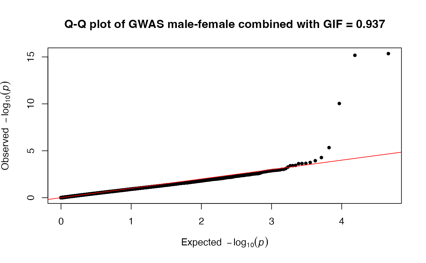
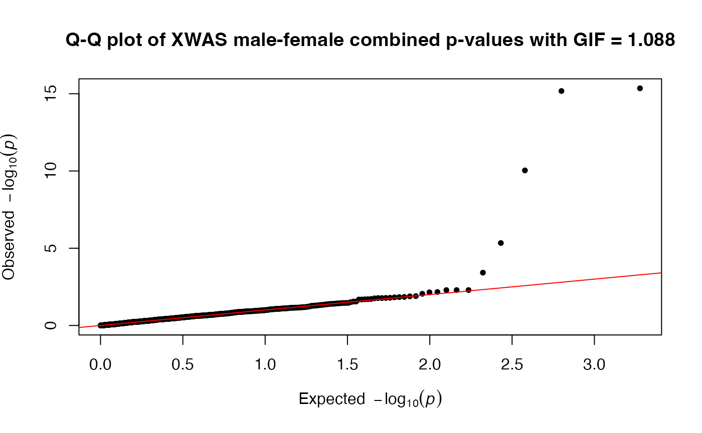
A dataframe with GWAS (with XWAS for X-chromosomal variants) along with Manhattan and Q-Q plots. In the case of the stratified test, the return is a list containing three dataframes, namely, FWAS, MWAS, and MFWAS with association results in only female, only male, and both cohorts, respectively. This will be accompanied by Miami and Q-Q plots. The individual manhattan and Q-Q-plots for stratified tests prefixed with xmodel type will be in the DataDir.

Author(s)

Banabithi Bose

References

Cinar O, Viechtbauer W (2022). “The poolr package for combining independent and dependent p values.” Journal of Statistical Software, 101(1), 1–42. doi:10.18637/jss.v101.i01.

Fisher RA (1925). Statistical Methods for Research Workers. Oliver and Boyd, Edinburgh.

Moreau Y, others (2003). “Comparison and meta-analysis of microarray data: from the bench to the computer desk.” Trends in Genetics, 19(10), 570–577.

Purcell S, Neale B, Todd-Brown K, Thomas L, Ferreira MAR, Bender D, Maller J, Sklar P, de Bakker PIW, Daly MJ, others (2007). “PLINK: A Tool Set for Whole-Genome Association and Population-Based Linkage Analyses.” The American Journal of Human Genetics, 81(3), 559–575. doi:10.1086/519795.

Rhodes DR (2002). “Meta-analysis of microarrays: interstudy validation of gene expression profiles reveals pathway dysregulation in prostate cancer.” Cancer Research, 62(15), 4427–4433.

Stouffer SA, Suchman EA, DeVinney LC, Star SA, Williams RM (1949). The American Soldier: Adjustment During Army Life, volume 1. Princeton University Press, Princeton, NJ.

Su Y, Hu J, Yin P, Jiang H, Chen S, Dai M, Chen Z, Wang P (2022). “XCMAX4: A Robust X Chromosomal Genetic Association Test Accounting for Covariates.” Genes (Basel), 13(5), 847. doi:10.3390/genes13050847, http://www.ncbi.nlm.nih.gov/pubmed/35627231.

Examples


DataDir <- GXwasR:::GXwasR_data()
ResultDir <- tempdir()
finput <- "GXwasR_example"
standard_beta <- TRUE
xsex <- FALSE
sex <- TRUE
Inphenocov <- NULL
covartest <- NULL
interaction <- FALSE
MF.na.rm <- FALSE
B <- 10000
MF.zero.sub <- 0.00001
trait <- "binary"
xmodel <- "FMcombx02"
combtest <- "fisher.method"
snp_pval <- 1e-08
covarfile <- NULL
ncores <- 0
MF.mc.cores <- 1
ResultGXwas <- GXwas(
    DataDir = DataDir, ResultDir = ResultDir,
    finput = finput, xmodel = xmodel, trait = trait, covarfile = covarfile,
    sex = sex, xsex = xsex, combtest = combtest, MF.p.corr = "none",
    snp_pval = snp_pval, plot.jpeg = TRUE, suggestiveline = 5, genomewideline = 7.3,
    MF.mc.cores = 1, ncores = ncores
)

Running GXwas

## Running
DataDir <- GXwasR:::GXwasR_data()
ResultDir <- tempdir()
finput <- "GXwasR_example"
standard_beta <- TRUE
xsex <- FALSE
sex <- TRUE
Inphenocov <- NULL
covartest <- NULL
interaction <- FALSE
MF.na.rm <- FALSE
B <- 10000
MF.zero.sub <- 0.00001
trait <- "binary"
xmodel <- "FMstratified"
combtest <- "fisher.method"
snp_pval <- 1e-08
covarfile <- NULL
ncores <- 2
plot.jpeg <- FALSE
MF.mc.cores <- 2
genomewideline <- 7.3
suggestiveline <- 5
plotname <- "GXwas.plot"
annotateTopSnp <- FALSE
MF.na.rm <- FALSE
B <- 10000
MF.zero.sub <- 0.00001
MF.p.corr <- "none"
plotname <- "GXwas.plot"
ResultGXwas <- GXwas(DataDir = DataDir, ResultDir = ResultDir, finput = finput, xmodel = xmodel, trait = trait, covarfile = covarfile, sex = sex, xsex = xsex, combtest = combtest, MF.p.corr = "none", snp_pval = snp_pval, plot.jpeg = plot.jpeg, suggestiveline = 5, genomewideline = 7.3, MF.mc.cores = 1, ncores = ncores)
#> • Running FMstratified model
#> Using PLINK v1.9.0-b.7.7 64-bit (22 Oct 2024)
#> • Stratified test is running for females
#> • Stratified test is running for males
#> • Parallel computation is in progress --------->
#> • Parallel computation is in progress --------->
#> ℹ Plots are initiated.
#> ℹ Saving plot to /var/folders/d6/gtwl3_017sj4pp14fbfcbqjh0000gp/T//RtmpMk2a8D/Stratified_GWAS.png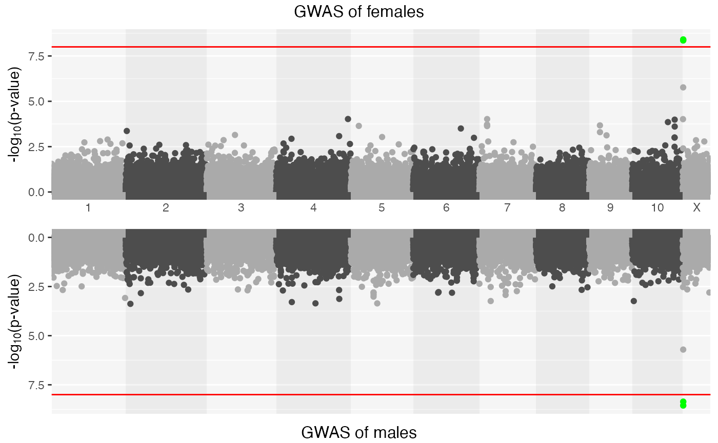

#> ℹ Saving plot to
#> /var/folders/d6/gtwl3_017sj4pp14fbfcbqjh0000gp/T//RtmpMk2a8D/Stratified_XWAS.png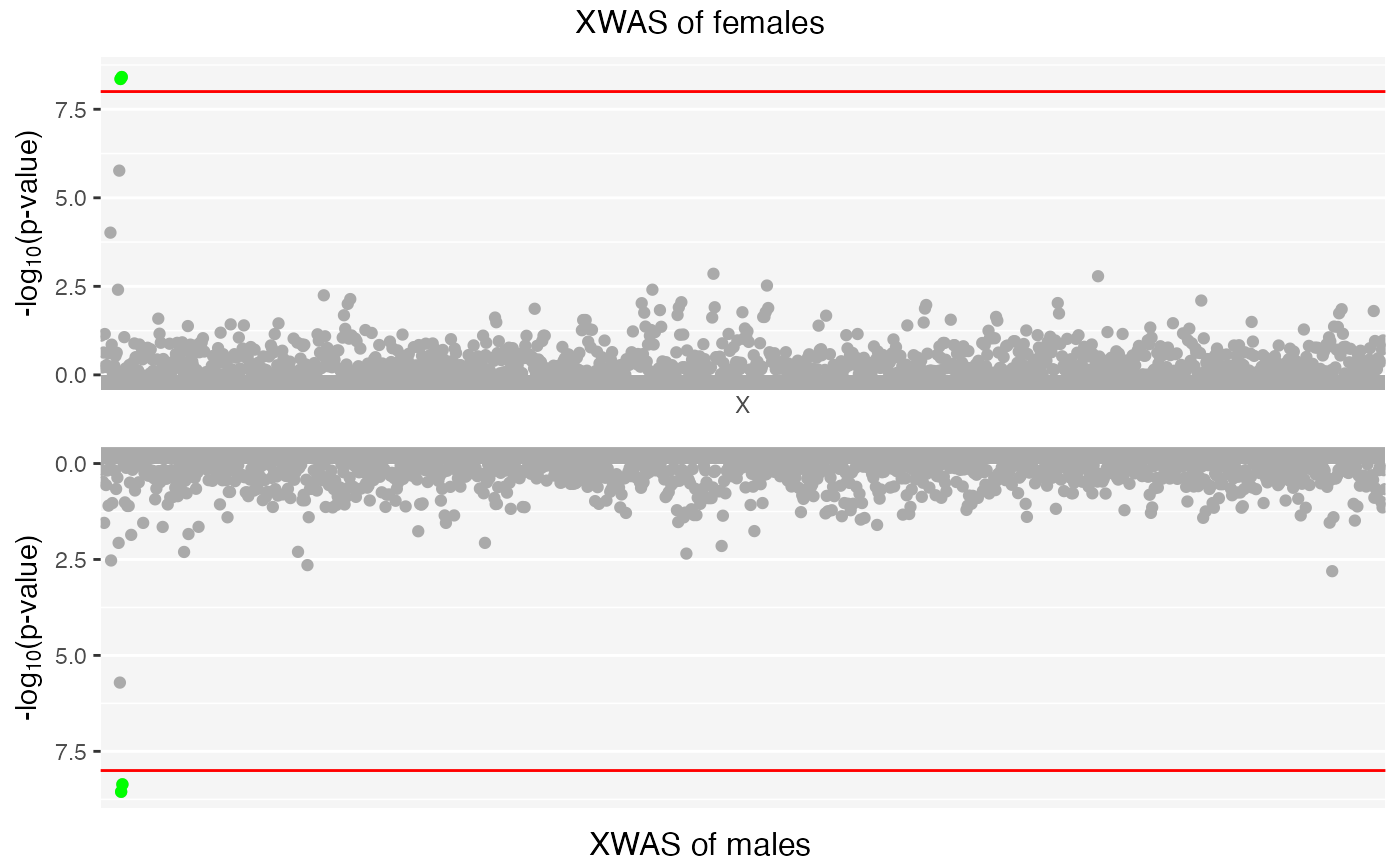

#> Three data frames have been created and saved:
#> • CombinedWAS
#> • MaleWAS
#> • FemaleWAS
#> ℹ You can find them in the directory: /var/folders/d6/gtwl3_017sj4pp14fbfcbqjh0000gp/T//RtmpMk2a8D

# Outputs
knitr::kable(ResultGXwas$CombinedWAS[1:5, ], caption = "Dataframe containing the result of stratified model")

Dataframe containing the result of stratified model
SNP	CHR	BP	P
rs10000405	4	47716881	0.9768464
rs10000452	4	63234460	0.6969710
rs10000465	4	120835814	0.5378310
rs10000605	4	13875675	0.7221672
rs10000675	4	121520624	0.8246220

knitr::kable(ResultGXwas$MaleWAS[1:5, ], caption = "Stratified GWAS result with male cohort.")

Stratified GWAS result with male cohort.
CHR	SNP	BP	A1	TEST	NMISS	BETA	SE	L95	U95	STAT	P
1	rs143773730	73841	T	ADD	125	-0.0789	0.2643	-0.5968	0.4390	-0.2986	0.76530
1	rs147281566	775125	T	ADD	125	-0.3959	1.2380	-2.8230	2.0310	-0.3197	0.74920
1	rs35854196	863863	A	ADD	125	1.0500	0.8858	-0.6864	2.7860	1.1850	0.23600
1	rs12041521	1109154	A	ADD	125	-0.4451	0.3387	-1.1090	0.2188	-1.3140	0.18890
1	rs148527527	1127860	G	ADD	125	1.6770	0.6864	0.3317	3.0220	2.4430	0.01456

knitr::kable(ResultGXwas$FemaleWAS[1:5, ], caption = "Stratified GWAS result with female cohort.")

Stratified GWAS result with female cohort.
CHR	SNP	BP	A1	TEST	NMISS	BETA	SE	L95	U95	STAT	P
1	rs143773730	73841	T	ADD	151	0.3459	0.2818	-0.2064	0.89820	1.2270	0.21970
1	rs147281566	775125	T	ADD	151	0.1568	0.9290	-1.6640	1.97800	0.1688	0.86590
1	rs35854196	863863	A	ADD	151	-0.1446	0.7282	-1.5720	1.28300	-0.1985	0.84260
1	rs115490086	928969	T	ADD	151	0.5649	1.4240	-2.2270	3.35700	0.3966	0.69170
1	rs12041521	1109154	A	ADD	151	-0.6697	0.3314	-1.3190	-0.02008	-2.0210	0.04332

## Top ten associations in female-specific study:
load(file.path(ResultDir, "FemaleWAS.Rda"))
x1 <- FemaleWAS
x2 <- x1[x1$TEST == "ADD", ]
x3 <- x2[order(x2$P), ]
x <- x3[1:10, -c(5:6)]
x

CHR	SNP	BP	A1	BETA	SE	L95	U95	STAT	P
23	rs12858640	4214861	C	-2.2040	0.3742	-2.9370	-1.4700	-5.889	0.0000000
23	rs6529954	4184349	A	-2.2050	0.3757	-2.9410	-1.4680	-5.868	0.0000000
23	rs5962098	4137114	A	1.4450	0.3019	0.8531	2.0370	4.785	0.0000017
4	rs7663144	186054771	C	-1.1510	0.2949	-1.7290	-0.5732	-3.904	0.0000947
7	rs4719409	14564068	G	0.9528	0.2442	0.4742	1.4310	3.902	0.0000955
23	rs6420571	3376304	A	-1.4560	0.3733	-2.1880	-0.7242	-3.900	0.0000963
10	rs11197338	117362943	A	-1.0370	0.2669	-1.5600	-0.5135	-3.884	0.0001027
10	rs2071426	96828323	C	-1.2900	0.3389	-1.9540	-0.6262	-3.808	0.0001402
7	rs2052980	14490891	A	-0.9751	0.2614	-1.4870	-0.4629	-3.731	0.0001908
9	rs4636286	22338570	G	0.9368	0.2529	0.4411	1.4330	3.704	0.0002124

## Top ten associations in male-specific study:
load(file.path(ResultDir, "MaleWAS.Rda"))
x1 <- MaleWAS
x2 <- x1[x1$TEST == "ADD", ]
x3 <- x2[order(x2$P), ]
x <- x3[1:10, -c(5:6)]
x

CHR	SNP	BP	A1	BETA	SE	L95	U95	STAT	P
23	rs6529954	4184349	A	-3.014	0.5071	-4.0080	-2.0200	-5.943	0.0000000
23	rs12858640	4214861	C	-2.838	0.4836	-3.7860	-1.8900	-5.870	0.0000000
23	rs5962098	4137114	A	1.924	0.4045	1.1320	2.7170	4.758	0.0000020
2	rs4669726	11531135	G	1.033	0.2926	0.4594	1.6060	3.530	0.0004154
5	rs73135224	76494977	T	1.025	0.2914	0.4534	1.5960	3.516	0.0004386
4	rs6820913	99125659	C	2.083	0.5927	0.9212	3.2450	3.514	0.0004410
4	rs2376095	36719306	A	1.017	0.2926	0.4432	1.5900	3.475	0.0005113
7	rs2270107	22862183	A	1.051	0.3054	0.4528	1.6500	3.442	0.0005764
10	rs2814902	3249289	G	1.051	0.3054	0.4528	1.6500	3.442	0.0005764
4	rs13149649	164553354	C	-1.000	0.2965	-1.5810	-0.4192	-3.374	0.0007418

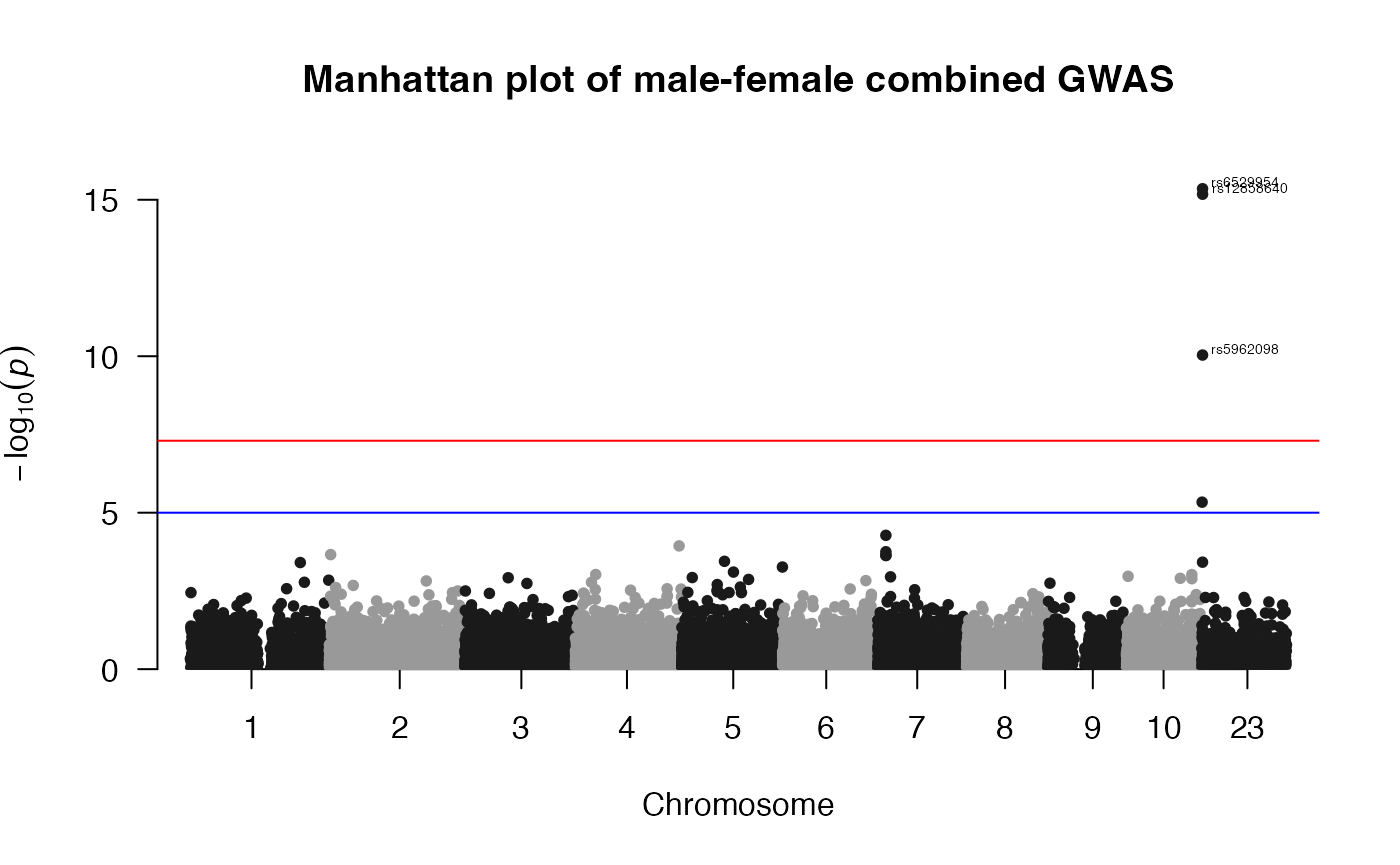
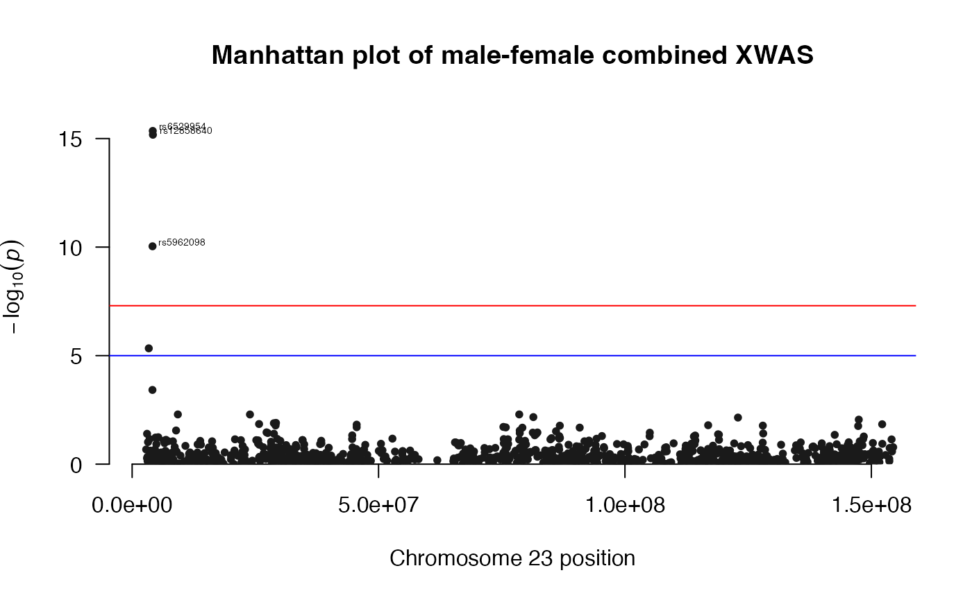
## Top ten associations in FM02comb model:
load(file.path(ResultDir, "CombinedWAS.Rda"))
x1 <- CombinedWAS
x2 <- x1[order(x1$P), ]
x <- x2[1:10, ]
x

SNP	CHR	BP	P
rs6529954	23	4184349	0.0000000
rs12858640	23	4214861	0.0000000
rs5962098	23	4137114	0.0000000
rs6420571	23	3376304	0.0000046
rs2052980	7	14490891	0.0000529
rs7663144	4	186054771	0.0001151
rs7794969	7	14518278	0.0001773
rs10186455	2	2579014	0.0002186
rs7801624	7	14528215	0.0002286
rs4719409	7	14564068	0.0002346

To know more about the function GXwas() to run different GWAS and XWAS models with different arguments, please follow this tutorial: https://boseb.github.io/GXwasR/articles/GXwasR_overview.html

Performing sex-differential test

Now, we will perform a sex-differential test:

Function: SexDiff()

help(SexDiff, package = GXwasR)

SexDiff

R Documentation

SexDiff: Sex difference in effect size for each SNP using t-test.

Description

This function uses the GWAS summary statistics from sex-stratified tests like "FMstratified", to evaluate the difference in effect size between males and females at each SNP using a t-test.

The input dataframes should only include X-chromosome in order to obtain results for sex differences based solely on X-linked loci.

Usage

SexDiff(Mfile, Ffile)

Arguments

Mfile

R dataframe of summary statistics of GWAS or XWAS of male samples with six mandatory columns, SNP(Variant),CHR(Chromosome number), BP(Base pair position),A1(Minor allele),BETA_M(Effect size) and SE_M(Standard error). This can be generated by running FM01comb or "FMstratified" model with GXWAS function.

Ffile

R dataframe of summary statistics of GWAS or XWAS of male samples with six mandatory columns, SNP(Variant),CHR(Chromosome number), BP(Base pair position),A1(Minor allele),BETA_F(Effect size) and SE_F(Standard error). This can be generated by running FM01comb or "FMstratified" model with GXWAS function.

Value

R dataframe with seven columns:

SNP (Variant)
CHR (Chromosome number)
BP (Base pair position)
A1 (Minor allele)
tstat (t-statistics for effect-size test)
P (p-value) and
adjP (Bonferroni corrected p-value)

Author(s)

Banabithi Bose

Examples

data("Mfile", package = "GXwasR")
data("Ffile", package = "GXwasR")
Difftest <- SexDiff(Mfile, Ffile)
significant_snps <- Difftest[Difftest$adjP < 0.05, ]

Running SexDiff

## Running
## Running the function
x1 <- MaleWAS
x1 <- x1[x1$TEST == "ADD", ]
x1 <- x1[, c(1:4, 7:8)]
colnames(x1) <- c("CHR", "SNP", "BP", "A1", "BETA_M", "SE_M")
x2 <- FemaleWAS
x2 <- x2[x2$TEST == "ADD", ]
x2 <- x2[, c(1:4, 7:8)]
colnames(x2) <- c("CHR", "SNP", "BP", "A1", "BETA_F", "SE_F")
Difftest <- SexDiff(Mfile = x1, Ffile = x2)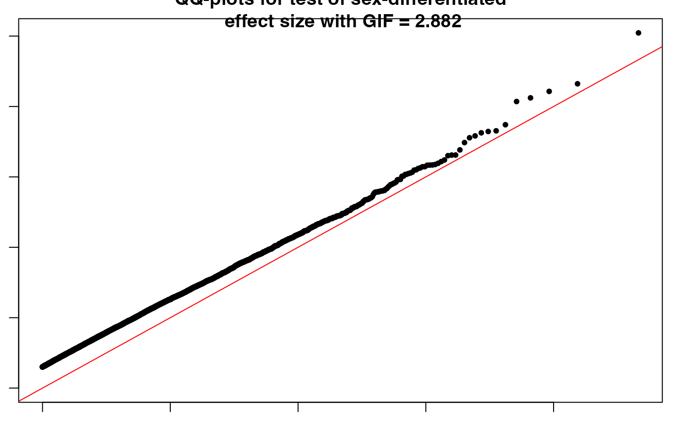

## Significant SNPs with sex-differential effect
sig.snps <- Difftest[Difftest$adjP < 0.05, ]
colnames(sig.snps) <- c("SNP", "CHR", "BP", "A1", "T_statistic", "Pvalue", "Adjusted_Pvalue")
if (nrow(sig.snps) > 0) {
  knitr::kable(sig.snps, caption = "SNPs with significant sex-differential effect.")
} else {
  message("No SNPs with significant sex-differential effect were found.")
}
#> No SNPs with significant sex-differential effect were found.

Citing `GXwasR`

We hope that GXwasR will be useful for your research. Please use the following information to cite the package and the overall approach. Thank you!

## Citation info
citation("GXwasR")
#> To cite package 'GXwasR' in publications use:
#> 
#>   Bose B, Blostein F, Kim J, Winters J, Actkins KV, Mayer D, Congivaram
#>   H, Niarchou M, Edwards DV, Davis LK, Stranger BE (2025). "GXwasR: A
#>   Toolkit for Investigating Sex-Differentiated Genetic Effects on
#>   Complex Traits." _medRxiv 2025.06.10.25329327_.
#>   doi:10.1101/2025.06.10.25329327
#>   <https://doi.org/10.1101/2025.06.10.25329327>.
#> 
#> A BibTeX entry for LaTeX users is
#> 
#>   @Article{,
#>     title = {GXwasR: A Toolkit for Investigating Sex-Differentiated Genetic Effects on Complex Traits},
#>     author = {Banabithi Bose and Freida Blostein and Jeewoo Kim and Jessica Winters and Ky’Era V. Actkins and David Mayer and Harrsha Congivaram and Maria Niarchou and Digna Velez Edwards and Lea K. Davis and Barbara E. Stranger},
#>     journal = {medRxiv 2025.06.10.25329327},
#>     year = {2025},
#>     doi = {10.1101/2025.06.10.25329327},
#>   }

Reproducibility

The GXwasR package (Bose, Blostein, Kim, Winters, Actkins, Mayer, Congivaram, Niarchou, Edwards, Davis, and Stranger, 2025) was made possible thanks to:

R (R Core Team, 2025)
BiocStyle (Oleś, 2025)
knitr (Xie, 2025)
RefManageR (McLean, 2017)
rmarkdown (Allaire, Xie, Dervieux, McPherson, Luraschi, Ushey, Atkins, Wickham, Cheng, Chang, and Iannone, 2025)
sessioninfo (Wickham, Chang, Flight, Müller, and Hester, 2025)
testthat (Wickham, 2011)

This package was developed using biocthis.

R session information.

#> ─ Session info ───────────────────────────────────────────────────────────────────────────────────────────────────────
#>  setting  value
#>  version  R version 4.5.1 (2025-06-13)
#>  os       macOS Sequoia 15.7.1
#>  system   aarch64, darwin24.4.0
#>  ui       unknown
#>  language en-US
#>  collate  en_US.UTF-8
#>  ctype    en_US.UTF-8
#>  tz       America/New_York
#>  date     2025-10-16
#>  pandoc   3.6.3 @ /Applications/Positron.app/Contents/Resources/app/quarto/bin/tools/aarch64/ (via rmarkdown)
#>  quarto   1.8.25 @ /usr/local/bin/quarto
#> 
#> ─ Packages ───────────────────────────────────────────────────────────────────────────────────────────────────────────
#>  package              * version   date (UTC) lib source
#>  abind                  1.4-8     2024-09-12 [1] CRAN (R 4.5.0)
#>  backports              1.5.0     2024-05-23 [1] CRAN (R 4.5.1)
#>  bibtex                 0.5.1     2023-01-26 [1] CRAN (R 4.5.0)
#>  bigassertr             0.1.7     2025-06-27 [1] CRAN (R 4.5.1)
#>  bigparallelr           0.3.2     2021-10-02 [1] CRAN (R 4.5.0)
#>  bigsnpr                1.12.21   2025-08-21 [1] CRAN (R 4.5.1)
#>  bigsparser             0.7.3     2024-09-06 [1] CRAN (R 4.5.1)
#>  bigstatsr              1.6.2     2025-07-29 [1] CRAN (R 4.5.1)
#>  Biobase                2.68.0    2025-04-15 [1] Bioconduc~
#>  BiocGenerics           0.54.0    2025-04-15 [1] Bioconduc~
#>  BiocIO                 1.18.0    2025-04-15 [1] Bioconduc~
#>  BiocManager            1.30.26   2025-06-05 [1] CRAN (R 4.5.0)
#>  BiocParallel           1.42.2    2025-09-14 [1] Bioconductor 3.21 (R 4.5.1)
#>  BiocStyle            * 2.36.0    2025-04-15 [1] Bioconduc~
#>  Biostrings             2.76.0    2025-04-15 [1] Bioconduc~
#>  bit                    4.6.0     2025-03-06 [1] CRAN (R 4.5.1)
#>  bit64                  4.6.0-1   2025-01-16 [1] CRAN (R 4.5.1)
#>  bitops                 1.0-9     2024-10-03 [1] CRAN (R 4.5.0)
#>  bookdown               0.45      2025-10-03 [1] CRAN (R 4.5.1)
#>  broom                  1.0.10    2025-09-13 [1] CRAN (R 4.5.1)
#>  BSgenome               1.76.0    2025-04-15 [1] Bioconduc~
#>  bslib                  0.9.0     2025-01-30 [1] CRAN (R 4.5.0)
#>  cachem                 1.1.0     2024-05-16 [1] CRAN (R 4.5.0)
#>  calibrate              1.7.7     2020-06-19 [1] CRAN (R 4.5.0)
#>  car                    3.1-3     2024-09-27 [1] CRAN (R 4.5.0)
#>  carData                3.0-5     2022-01-06 [1] CRAN (R 4.5.0)
#>  cli                    3.6.5     2025-04-23 [1] CRAN (R 4.5.0)
#>  codetools              0.2-20    2024-03-31 [3] CRAN (R 4.5.1)
#>  cowplot                1.2.0     2025-07-07 [1] CRAN (R 4.5.1)
#>  crayon                 1.5.3     2024-06-20 [1] CRAN (R 4.5.0)
#>  curl                   7.0.0     2025-08-19 [1] CRAN (R 4.5.1)
#>  data.table             1.17.8    2025-07-10 [1] CRAN (R 4.5.1)
#>  DelayedArray           0.34.1    2025-04-17 [1] Bioconduc~
#>  desc                   1.4.3     2023-12-10 [1] CRAN (R 4.5.0)
#>  digest                 0.6.37    2024-08-19 [1] CRAN (R 4.5.0)
#>  doParallel             1.0.17    2022-02-07 [1] CRAN (R 4.5.0)
#>  doRNG                  1.8.6.2   2025-04-02 [1] CRAN (R 4.5.0)
#>  dplyr                  1.1.4     2023-11-17 [1] CRAN (R 4.5.0)
#>  evaluate               1.0.5     2025-08-27 [1] CRAN (R 4.5.1)
#>  farver                 2.1.2     2024-05-13 [1] CRAN (R 4.5.0)
#>  fastmap                1.2.0     2024-05-15 [1] CRAN (R 4.5.0)
#>  flock                  0.7       2016-11-12 [1] CRAN (R 4.5.1)
#>  foreach                1.5.2     2022-02-02 [1] CRAN (R 4.5.0)
#>  Formula                1.2-5     2023-02-24 [1] CRAN (R 4.5.0)
#>  fs                     1.6.6     2025-04-12 [1] CRAN (R 4.5.0)
#>  gdsfmt                 1.44.1    2025-07-09 [1] Bioconduc~
#>  generics               0.1.4     2025-05-09 [1] CRAN (R 4.5.0)
#>  GenomeInfoDb           1.44.3    2025-09-21 [1] Bioconductor 3.21 (R 4.5.1)
#>  GenomeInfoDbData       1.2.14    2025-04-21 [1] Bioconductor
#>  GenomicAlignments      1.44.0    2025-04-15 [1] Bioconduc~
#>  GenomicRanges          1.60.0    2025-04-15 [1] Bioconduc~
#>  ggplot2                4.0.0     2025-09-11 [1] CRAN (R 4.5.1)
#>  ggpubr                 0.6.1     2025-06-27 [1] CRAN (R 4.5.1)
#>  ggrepel                0.9.6     2024-09-07 [1] CRAN (R 4.5.1)
#>  ggsignif               0.6.4     2022-10-13 [1] CRAN (R 4.5.0)
#>  glue                   1.8.0     2024-09-30 [1] CRAN (R 4.5.0)
#>  gridExtra              2.3       2017-09-09 [1] CRAN (R 4.5.0)
#>  gtable                 0.3.6     2024-10-25 [1] CRAN (R 4.5.0)
#>  GXwasR               * 0.99.0    2025-10-02 [1] Bioconductor
#>  hms                    1.1.3     2023-03-21 [1] CRAN (R 4.5.0)
#>  htmltools              0.5.8.1   2024-04-04 [1] CRAN (R 4.5.0)
#>  htmlwidgets            1.6.4     2023-12-06 [1] CRAN (R 4.5.0)
#>  httr                   1.4.7     2023-08-15 [1] CRAN (R 4.5.0)
#>  IRanges                2.42.0    2025-04-15 [1] Bioconduc~
#>  iterators              1.0.14    2022-02-05 [1] CRAN (R 4.5.0)
#>  jquerylib              0.1.4     2021-04-26 [1] CRAN (R 4.5.0)
#>  jsonlite               2.0.0     2025-03-27 [1] CRAN (R 4.5.0)
#>  knitr                  1.50      2025-03-16 [1] CRAN (R 4.5.0)
#>  labeling               0.4.3     2023-08-29 [1] CRAN (R 4.5.0)
#>  lattice                0.22-7    2025-04-02 [3] CRAN (R 4.5.1)
#>  lifecycle              1.0.4     2023-11-07 [1] CRAN (R 4.5.0)
#>  lubridate              1.9.4     2024-12-08 [1] CRAN (R 4.5.1)
#>  magrittr               2.0.4     2025-09-12 [1] CRAN (R 4.5.1)
#>  MASS                   7.3-65    2025-02-28 [3] CRAN (R 4.5.1)
#>  mathjaxr               1.8-0     2025-04-30 [1] CRAN (R 4.5.1)
#>  Matrix                 1.7-4     2025-08-28 [3] CRAN (R 4.5.1)
#>  MatrixGenerics         1.20.0    2025-04-15 [1] Bioconduc~
#>  matrixStats            1.5.0     2025-01-07 [1] CRAN (R 4.5.0)
#>  memoise                2.0.1     2021-11-26 [1] CRAN (R 4.5.0)
#>  pillar                 1.11.1    2025-09-17 [1] CRAN (R 4.5.1)
#>  pkgconfig              2.0.3     2019-09-22 [1] CRAN (R 4.5.0)
#>  pkgdown                2.1.3     2025-05-25 [2] CRAN (R 4.5.0)
#>  plyr                   1.8.9     2023-10-02 [1] CRAN (R 4.5.1)
#>  plyranges              1.28.0    2025-04-15 [1] Bioconduc~
#>  poolr                  1.2-0     2025-05-07 [1] CRAN (R 4.5.0)
#>  prettyunits            1.2.0     2023-09-24 [1] CRAN (R 4.5.0)
#>  printr               * 0.3       2023-03-08 [1] CRAN (R 4.5.0)
#>  progress               1.2.3     2023-12-06 [1] CRAN (R 4.5.0)
#>  purrr                  1.1.0     2025-07-10 [1] CRAN (R 4.5.1)
#>  qqman                  0.1.9     2023-08-23 [1] CRAN (R 4.5.0)
#>  R.methodsS3            1.8.2     2022-06-13 [1] CRAN (R 4.5.0)
#>  R.oo                   1.27.1    2025-05-02 [1] CRAN (R 4.5.0)
#>  R.utils                2.13.0    2025-02-24 [1] CRAN (R 4.5.0)
#>  R6                     2.6.1     2025-02-15 [1] CRAN (R 4.5.0)
#>  ragg                   1.5.0     2025-09-02 [2] CRAN (R 4.5.1)
#>  rbibutils              2.3       2024-10-04 [1] CRAN (R 4.5.1)
#>  RColorBrewer           1.1-3     2022-04-03 [1] CRAN (R 4.5.0)
#>  Rcpp                   1.1.0     2025-07-02 [1] CRAN (R 4.5.1)
#>  RCurl                  1.98-1.17 2025-03-22 [1] CRAN (R 4.5.0)
#>  Rdpack                 2.6.4     2025-04-09 [1] CRAN (R 4.5.0)
#>  RefManageR           * 1.4.0     2022-09-30 [1] CRAN (R 4.5.1)
#>  regioneR               1.40.1    2025-06-01 [1] Bioconductor 3.21 (R 4.5.0)
#>  restfulr               0.0.16    2025-06-27 [1] CRAN (R 4.5.1)
#>  rjson                  0.2.23    2024-09-16 [1] CRAN (R 4.5.0)
#>  rlang                  1.1.6     2025-04-11 [1] CRAN (R 4.5.0)
#>  rmarkdown            * 2.30      2025-09-28 [1] CRAN (R 4.5.1)
#>  rmio                   0.4.0     2022-02-17 [1] CRAN (R 4.5.0)
#>  rngtools               1.5.2     2021-09-20 [1] CRAN (R 4.5.0)
#>  Rsamtools              2.24.1    2025-09-07 [1] Bioconductor 3.21 (R 4.5.1)
#>  rstatix                0.7.2     2023-02-01 [1] CRAN (R 4.5.0)
#>  rtracklayer            1.68.0    2025-04-15 [1] Bioconduc~
#>  S4Arrays               1.8.1     2025-06-01 [1] Bioconductor 3.21 (R 4.5.0)
#>  S4Vectors              0.46.0    2025-04-15 [1] Bioconduc~
#>  S7                     0.2.0     2024-11-07 [1] CRAN (R 4.5.1)
#>  sass                   0.4.10    2025-04-11 [1] CRAN (R 4.5.0)
#>  scales                 1.4.0     2025-04-24 [1] CRAN (R 4.5.0)
#>  sessioninfo          * 1.2.3     2025-02-05 [1] CRAN (R 4.5.1)
#>  SNPRelate              1.42.0    2025-04-15 [1] Bioconduc~
#>  SparseArray            1.8.1     2025-07-23 [1] Bioconduc~
#>  stringi                1.8.7     2025-03-27 [1] CRAN (R 4.5.0)
#>  stringr                1.5.2     2025-09-08 [1] CRAN (R 4.5.1)
#>  sumFREGAT              1.2.5     2022-06-07 [1] CRAN (R 4.5.1)
#>  SummarizedExperiment   1.38.1    2025-04-30 [1] Bioconductor 3.21 (R 4.5.0)
#>  sys                    3.4.3     2024-10-04 [1] CRAN (R 4.5.0)
#>  systemfonts            1.3.1     2025-10-01 [1] CRAN (R 4.5.1)
#>  textshaping            1.0.3     2025-09-02 [1] CRAN (R 4.5.1)
#>  tibble                 3.3.0     2025-06-08 [1] CRAN (R 4.5.0)
#>  tidyr                  1.3.1     2024-01-24 [1] CRAN (R 4.5.1)
#>  tidyselect             1.2.1     2024-03-11 [1] CRAN (R 4.5.0)
#>  timechange             0.3.0     2024-01-18 [1] CRAN (R 4.5.1)
#>  tzdb                   0.5.0     2025-03-15 [1] CRAN (R 4.5.1)
#>  UCSC.utils             1.4.0     2025-04-15 [1] Bioconduc~
#>  vctrs                  0.6.5     2023-12-01 [1] CRAN (R 4.5.0)
#>  vroom                  1.6.6     2025-09-19 [1] CRAN (R 4.5.1)
#>  withr                  3.0.2     2024-10-28 [1] CRAN (R 4.5.0)
#>  xfun                   0.53      2025-08-19 [1] CRAN (R 4.5.1)
#>  XML                    3.99-0.19 2025-08-22 [1] CRAN (R 4.5.1)
#>  xml2                   1.4.0     2025-08-20 [1] CRAN (R 4.5.1)
#>  XVector                0.48.0    2025-04-15 [1] Bioconduc~
#>  yaml                   2.3.10    2024-07-26 [1] CRAN (R 4.5.0)
#> 
#>  [1] /Users/mayerdav/Library/R/arm64/4.5/library
#>  [2] /opt/homebrew/lib/R/4.5/site-library
#>  [3] /opt/homebrew/Cellar/r/4.5.1/lib/R/library
#>  * ── Packages attached to the search path.
#> 
#> ──────────────────────────────────────────────────────────────────────────────────────────────────────────────────────

Bibliography

This vignette was generated using BiocStyle (Oleś, 2025) with knitr (Xie, 2025) and rmarkdown (Allaire, Xie, Dervieux et al., 2025) running behind the scenes.

Citations made with RefManageR (McLean, 2017).

[1] J. Allaire, Y. Xie, C. Dervieux, et al. rmarkdown: Dynamic Documents for R. R package version 2.30. 2025. URL: https://github.com/rstudio/rmarkdown.

[2] B. Bose, F. Blostein, J. Kim, et al. “GXwasR: A Toolkit for Investigating Sex-Differentiated Genetic Effects on Complex Traits”. In: medRxiv 2025.06.10.25329327 (2025). DOI: 10.1101/2025.06.10.25329327.

[3] M. W. McLean. “RefManageR: Import and Manage BibTeX and BibLaTeX References in R”. In: The Journal of Open Source Software (2017). DOI: 10.21105/joss.00338.

[4] A. Oleś. BiocStyle: Standard styles for vignettes and other Bioconductor documents. R package version 2.36.0. 2025. DOI: 10.18129/B9.bioc.BiocStyle. URL: https://bioconductor.org/packages/BiocStyle.

[5] R Core Team. R: A Language and Environment for Statistical Computing. R Foundation for Statistical Computing. Vienna, Austria, 2025. URL: https://www.R-project.org/.

[6] H. Wickham. “testthat: Get Started with Testing”. In: The R Journal 3 (2011), pp. 5–10. URL: https://journal.r-project.org/archive/2011-1/RJournal_2011-1_Wickham.pdf.

[7] H. Wickham, W. Chang, R. Flight, et al. sessioninfo: R Session Information. R package version 1.2.3. 2025. DOI: 10.32614/CRAN.package.sessioninfo. URL: https://CRAN.R-project.org/package=sessioninfo.

[8] Y. Xie. knitr: A General-Purpose Package for Dynamic Report Generation in R. R package version 1.50. 2025. URL: https://yihui.org/knitr/.

Banabithi Bose

16 October 2025

Introduction

Example Datasets

Loading the GXwasR library

Learn about all the GXwasR functions

Example Dataset Summary

Sex-combined and sex-stratified GWAS with XWAS

Function: GXwas()

GXwas: Running genome-wide association study (GWAS) and X-chromosome-wide association study (XWAS) models.

Description

Usage

Arguments

Value

Author(s)

References

Examples

Running GXwas

Performing sex-differential test

Function: SexDiff()

SexDiff: Sex difference in effect size for each SNP using t-test.

Description

Usage

Arguments

Value

Author(s)

Examples

Running SexDiff

Citing GXwasR

Reproducibility

Bibliography

Citing `GXwasR`